The conductance and current-voltage relationships of molecular junctions can be calculated using either Landauer or Non-Equilibrium Green’s Function (NEGF) levels of theory. In both cases, the Green’s function formulation is employed using a chosen electronic structure level. See Refs. 251, 269 for further introduction.
In molecular junctions the current-voltage curve depends on the electron transmission function, which can be calculated using the quantum transport code developed by the Dunietz group (Kent State). The scattering-free approach, (Landauer), provides a zero-bias limit, the non-equilibrium approach, (NEGF), provides a voltage-dependent transmission by solving iteratveily for the bias-affected electronic density.
This quantum transport utility is invoked by setting the $rem variable TRANS_ENABLE.
TRANS_ENABLE
To invoke the molecular transport code.
INPUT SECTION: $REM
TYPE:
INTEGER
DEFAULT:
0
OPTIONS:
0
Do not perform electron transport calculation.
1
Landauer; zero bias limit.
3
A self-consistent Green’s function calculation at zero bias voltage
(NEGF with zero bias, typically used for preparation of bias dependent NEGF).
4
Full NEGF.
-1
Print matrices needed for generating bulk model data files.
RECOMMENDATION:
Values 3 or 4 must be set with SCF_ALGORITHM = NEGF in the $rem section and should set
SYM_IGNORE = TRUE to fix the atomic coordinates.
For NEGF calculations, the transport axis is assumed to be along X axis, along which the bias potential is dropped.
In addition to information included in the Q-Chem output file the following files are generated:
transmission.txt (Transmission function in the requested energy window)
TDOS.txt (Total density of states)
current.txt (I-V plot only for the Landauer level)
IV-NEGF-all.txt (I-V plot obtained by NEGF method)
The transport flag can be used to print out data matrices of the junction or the bulk models that can be used in subsequent transport calculations:
FAmat.dat (Hamiltonian matrix for follow up calculations and analysis)
Smat.dat (Overlap matrix for follow up calculations and analysis)
DAmat.dat (Density matrix for follow up calculations and analysis [only for NEGF])
(In case of printing bulk information the files need to be renamed as explained below.)
In the case of unrestricted spin the output file names are appended by A[B] to indicate the spin state. (e.g. transmissionA.txt and transmissionB.txt). We note that in the closed-shell spin-restricted case, the transmission.txt corresponds to the spin, where the total transmission due to the spin symmetry is twice the values included in the file.
The Landauer level generates a single set of output files. NEGF calculation provides directories for the different biases where the directories Vbias1, Vbias2, (the numbers in the directory names are used to index the bias voltage) contain the output files at the corresponding bias.
The T-Chem program allows for large flexibility in setting up the transport calculation and therefore requires setting several parameters. Accordingly, the actual molecular junction model is partitioned into domains representing the electrode self-energy (SEs) and the central bridge region, and the procedure by which the SEs are calculated.
This setup is addressed in two transport-specific sections in the input file:
$trans_model (molecular junction regions)
$trans_method (sets various transport flags include details for the SE evaluation, NEGF integration, grid parameters, and various input parameters as the Fermi energy and the bias.)
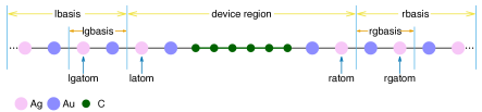
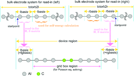
The $trans_model section partitions the molecular model, assigning the atomic basis functions to different regions. There are no default values. The different regions are set as illustated in Fig. 13.1 and Fig. 13.2 for the Landauer and NEGF levels, respectively.
The parameters in the $trans_model section can be provided either in terms of the atom numbers or basis functions. Note: Only one set of these numbers is required. The assignment based on trans_latom etc. has priority.
trans_latom: INTEGER, atom index, where the central/bridge region starts (the first atom in junction area).
trans_ratom: INTEGER, atom index, where the central/bridge region ends (the last atom in junction area).
trans_lgatom: INTEGER, atom index where the repeat unit of the left electrode starts.
trans_rgatom: INTEGER, atom index where the repeat unit of the right electrode ends.
Atoms within numbers trans_lgatom, trans_lgatom+1, .., trans_latom-1 define the repeat unit of the left electrode (similarly for right electrode).
trans_lbasis: INTEGER, the number of basis functions appearing to the left of the device region (the index of the first AO within the central region).
trans_rbasis: INTEGER, the number of basis functions appearing to the right of the device region right electrode (total number of basis functions minus this number equals last AO that is within the device).
trans_lgbasis: INTEGER, the number of basis functions of the repeat unit of the left electrode.
trans_rgbasis: INTEGER, the number of basis functions of the repeat unit of the right electrode.
For the NEGF calculation, trans_lbasis and trans_lgbasis must be the same number as shown in Fig. 13.2 (also for trans_rbasis and trans_rgbasis). The NEGF calculations require precalculated bulk data, while the Landauer can use such precalculated data as an option.
The example in Fig. 13.1 includes a total of 18 atoms, where the Au and Ag basis sets each contain 22 basis functions per atom. The repeat unit includes a pair of Au Ag atoms. Therefore, the parameters should be given as follows (only the first two columns are required, the rest are included for explanation):
| trans_lbasis | 88 | No. of functions representing left electrode region ( for Ag + for Au) |
|---|---|---|
| trans_rbasis | 88 | No. of functions representing right electrode ( for Ag + for Au) |
| trans_lgbasis | 44 | Size of the repeating unit of the left electrode (22 for Ag + 22 for Au) |
| trans_rgbasis | 44 | Size of the repeating unit of the right electrode (22 for Ag + 22 for Au) |
Alternatively this section can be based on the atom numbers corresponding to their position in the $molecule section:
| trans_lgatom | 3 | Third atom is used to define the repeat unit of the left electrode |
| trans_latom | 5 | Fifth atom is the first atom of the junction |
| trans_ratom | 14 | Fourteenth atom is the last atom of the junction |
| trans_rgatom | 16 | Sixteenth atom is used to define the repeat unit of the right electrode |
In this example, we have used the same repeat unit for the left and right electrodes; this symmetry is not required.
WARNING: In both illustrated examples atomic wires are used: Au/Ag wire in the Landauer case and Al wire for the NEGF example. Here The Au/Ag pair or a single Al atom represent a bulk repeat unit, in more detailed models it is essential that the atoms within the unit are introduced at the same order in all units. All bulk layers have to appear in order (”left to right”) including those units that are designated to be the first and last bulk unit included within the central region.
Note: The order of atoms in the $molecule section is important and assumes the following: Repeating units (left) - Molecular Junction - Repeating units (right)
The atoms are provided first by the leftmost repeat unit in the left electrode then proceeds to the next repeat unit up to the surface unit. Next the bridge atoms are provided followed by the right surface unit and the right electrode region. The right electrode region starts with the surface layer and ends with the most distant layer within the bulk. The atoms order within each of the included electrode repeat units must be consistent. The atoms order within the bridge region (excluding the electrode repeat unit atoms) is arbitrary.
That is, the order of atoms in the molecule section has to adhere to the following:
atoms of the leftmost repeat unit
atoms of the next repeat unit(s) (if avaialble)
atoms of the left surface unit device
bridge atoms
atoms of the right surface unit
atoms of the next right electrode unit(s) (if avaialble)
atoms of the rightmost repeat unit
T-Chem allows for complete flexibility in determining the different regions of the electrode models. As a consequence, incorrect setting of the regions cannot be caught by the program and may result in transmission functions that are unphysical (e.g. large or even negative values). Such errors can occur where the cluster model is partitioned (by mistake) within the orbital space of an atom. Regions should be defined between the repeat units. The atoms within each repeat unit must be always provided in the same internal order, and must be consistent with the order (and orientation!) used in the precalculation of the bulk model (if employed).
Note: At least a single repeat unit of the electrodes should be included in the bridge region. With the Landauer model, if trans_readhs == 0, then at least one unit beyond the bridge region has to be included, an additional unit (total of two at least) is required, when also trans_method != 0.
The necessary parameters in $trans_method section are listed as follows:
trans_spin
Spin coordinates.
INPUT SECTION: $trans_method
TYPE:
INTEGER
DEFAULT:
0
OPTIONS:
0
Restricted spin calculations or closed-shell singlet states.
3
Unrestricted spin calculations or open-shell systems (both spins are calculated).
RECOMMENDATION:
None
trans_method
Electrode surface GF model.
INPUT SECTION: $trans_method
TYPE:
INTEGER
DEFAULT:
0
OPTIONS:
0
A wide band limit (WBL) with a constant parameter trans_greens (default).
1
WBL using the Ke-Baranger-Yang TB at the Fermi energy.
2
WBL using the Lopez-Sancho TB at the Fermi energy.
3
Tight-binding (TB) following the Ke-Baranger-Yang algorithm.
4
TB following the Lopez-Sancho algorithm (decimation).
RECOMMENDATION:
Note: Only option 0 is currently available for NEGF calculations.
trans_readhs
Flag to read the Hamiltonian and overlap matrices of the bulk model.
INPUT SECTION: $trans_method
TYPE:
INTEGER
DEFAULT:
0
Use the current Hamiltonian and overlap matrices to parse out the electrode
matrices.
OPTIONS:
1
Use pre-calculated electrode Hamiltonian and overlap matrices. Required for NEGF.
RECOMMENDATION:
If set to 1, the following files are requred: FAmat2l.dat and
Smat2l.dat (for left electrode model), FAmat2r.dat and
Smat2r.dat (for right electrode model). If both electrodes are of the
same type, may use symbolic links to the same files. (For
unrestricted spin model, FBmat2l.dat and FBmat2r.dat are also
necessary)
For trans_readhs = 1, the paramters for parsing the precalculated bulk matrices ( FAmat2l.dat, etc) have to be provided. These indices define the regions within the bulk full model space to set the onsite and coupling matrcies for the SE calculations.
trans_totorb2 (Integer):
Total number of basis functions in the electrode models (if set, then
same size is assumed for both electrodes) (no default value).
trans_totorb2l: Integer number, total number of basis functions in left electrode model (no default value).
trans_totorb2r: Integer number, total number of basis functions in right electrode model (no default value).
trans_startpoint: Integer number, start point (basis number) for reading the TB integrals. Note, the basis number, that is, index number of basis function starts from 0. (if set, then same size is assumed for both electrodes) (default value 0).
trans_startpointl: given as integer number, left start point (basis number) for reading the TB integrals. Note, the basis number, that is, index number of basis function starts from 0. (default value 0).
trans_startpointr: given as integer number, right start point (basis number) for reading the TB integrals. Note, the basis number, that is, index number of basis function starts from 0. (no default value).
Note: NEGF requires trans_readhs to be set where SEs are precalculated. The Landauer level can obtain bulk parameters from the current job of a molecular junction model.
Options to control the output:
trans_npoint (Integer):
Number of grid points within the energy window of the transmission spectra
calculation.
300
Default value.
trans_printdos (Integer):
Controls the printout of TDOS.
0
Default, no total DOS printing.
1
A TDOS (of the junction region) will be printed to TDOS.txt (closed shell).
trans_printiv (Integer):
Calculated current (at the zero bias case).
0
Default, no current calculated and printed
1
Current will be printed to current.txt (closed shell) or
currentA/B.txt (unrestricted or open shell).
trans_ipoints (Integer):
Number of points for current calculation (at the zero bias case).
300
Default value.
The following parameters control the imaginary smearing in calculating GFs:
trans_greens (Double):
Imaginary smearing/Broadening (in eV) added to the surface Green’s function (only relevant for trans_method==0).
0.07
Default
trans_devsmear (Double):
Imaginary smearing (in eV) added to the real Hamiltonian in central region
retarded GF evaluation.
0.01
Default
trans_bulksmear (Double):
Imaginary smearing (in eV) added to the real Hamiltonian in electrodes GF
evaluation (relevant for trans_method>0).
0.01
Default
trans_efermi (Double):
Fermi energy of the electrode (for spin) (in eV) used for defining
the energy window of the T(E).
-5.0
Default
trans_efermib (Double):
Fermi energy for spin (in eV). If this is not given, the same value of
spin is used.
trans_adjustefermi (Integer):
Resetting of the Fermi energy (FE) in NEGF using trans_enable = 3 or 4
0
Default. Fixed FE specified by trans_efermi (and
trans_efermib) is used.
1
FE is chosen as midpoint of HOMO and LUMO levels
2
FE is adjusted so that charge neutrality is satisfied (recommended for zero bias calculation to establish the Fermi energy of the model)
Options 1, 2 use the same FE for and spins. Negative options allow for different FEs for and spins.
trans_vmax (Double):
Maximum voltage bias (V).
1.0
Default
Note: The default energy window for transmission and current calculations is defined as: trans_emin = trans_efermi - trans_vmax/2 and trans_emax = trans_efermi + trans_vmax/2 if trans_emin and trans_emax are not given.
The trans_emin and trans_emax values can be set to determine the energy window for calculating the transmission function (both must be specified). If specified, these values will override the window defined by trans_efermi and trans_vmax values.
The following paramter establish the voltages for the NEGF level (trans_enable==4):
trans_vstart (Double):
(Only for trans_enable = 4). Starting voltage bias (V). The bias
voltage increases from trans_vstart to
trans_vmax in the NEGF calculation.
0.0
Default
trans_nvbias (Integer):
(Only for trans_enable = 4), number of points of bias voltage.
1
Default
The bias voltage values to be calculated are defined by dividing the range
between trans_vstart and trans_vmax with this number. For
example, when trans_vstart = 0.0, trans_vmax = 1.0, and
trans_nvbias = 5, the voltages are 0.0, 0.25, 0.50, 0.75, and 1.0.
For the case of trans_nvbias = 1, the voltage to be calculated is
trans_vmax.
trans_gridoffset (Double):
(Only for trans_enable = 4),
Offset distance (in A) to define extended grid box size used for obtaining matrix elements that involve the electrostatic potential in the Fock matrix. See below for details.
5.0
Default
The bias voltage of is added on the left electrode, and on the right electrode, where the bias potential slope is along -axis. The offset should be set to the location of the left surface layer from the leftmost atom in the atomic coordinates (the first atom in the molecule section). The box size is defined by adding/substracting the offset distance to maximum/minimum of each of the , and atomic coordinates. The bias voltage on the grid points in the box is used for calculating correction term for the Fock matrix (i.e. ).
Note that this grid is not for obtaining electrostatic potential by solving the Poisson equation. The setup of the Poisson equation solver is described below. The grid for the Poisson equation is given by $plots block keyword (see also example below). The same grid size is used for both boxes.
The following are parameters for addressing the NEGF iterations, trans_enable = 3, 4:
trans_restart (Integer):
Flag to restart reading the density matrix files, DAmat.dat
(and DBmat.dat) from the "TransRestart/" directory.
0
No restart (default).
1
Read file of density matrix.
trans_mixing (Double):
Mixing ratio of DIIS mixing method for updating the central block of density
matrix in the NEGF iteration.
1.0
Default
trans_mixhistory (Integer):
The number of NEGF iteration steps in which the history of density matrix is
stored for the DIIS method.
40
Default
The following parameters are used to set the NEGF density integration:
trans_dehcir (Double):
Grid size, dE (in eV), for integrating the Greens function on the half circle
path on imaginary plane.
1.0
Default
trans_delpart (Double):
Grid size, dE (in eV), for integrating the Greens function on the path of the
linear part on imaginary plane.
0.01
Default
trans_debwin (Double):
(For trans_enable = 4). Grid size, dE (in eV), for integration on the
non-equilibrium term.
0.01
Default
trans_numres (Integer):
The number of poles at Fermi energy enclosed by the contour into the
imaginary plane.
100
Default
Parameters for controlling the electrostatic potential calculation, the Poisson solver:
trans_peconv (Integer):
The convergence criteria of the iteration of the Poisson equation. The
threshold is 10 hartree of maximum energy difference over the all grid
points.
9
Default
trans_pemaxite (Integer):
Maximum iterations of the Poisson solver.
1000
Default
trans_readesp (Integer):
Storing or reading in the electrostatic potential.
The data is stored in "ReadInESP/" directory.
-1
Write the ESP data to the "ReadInESP/" directory at the first step and
stop calculation.
0
Write the ESP data to the "ReadInESP/" at the first step and continue
calculation using it (default).
1
Read the pre-calculated read-in ESP data from "ReadInESP/" and continue
calculation.
As an example of the Landauer calculation, the sample Q-Chem input is given below.
Example 13.3 Quantum transport Landauer calculation applied to C between two gold electrodes.
$molecule
   0 1
   Ag   -11.000    0.000  0.000
   Au    -8.300    0.000  0.000
   Ag    -5.600    0.000  0.000
   Au    -2.900    0.000  0.000
   Ag    -0.200    0.000  0.000
   Au     2.500    0.000  0.000
   C      4.800    0.000  0.000
   C      6.500    0.000  0.000
   C      8.200    0.000  0.000
   C      9.900    0.000  0.000
   C     11.600    0.000  0.000
   C     13.300    0.000  0.000
   Au    15.600    0.000  0.000
   Ag    18.300    0.000  0.000
   Au    21.000    0.000  0.000
   Ag    23.700    0.000  0.000
   Au    26.400    0.000  0.000
   Ag    29.100    0.000  0.000
$end

$rem
   METHOD            B3LYP
   BASIS             lanl2dz
   ECP               lanl2dz
   ECP_FIT           true
   INCDFT            FALSE
   MOLDEN_FORMAT     TRUE
   SCF_CONVERGENCE   6
   TRANS_ENABLE      1
$end

$trans-method
   trans_spin        0
   trans_npoints     300
   trans_method      0
   trans_readhs      0
   trans_printdos    1
   trans_efermi      -6.50
   trans_vmax        4.00
$end

$trans-model
   trans_lgatom      3
   trans_latom       5
   trans_ratom       14
   trans_rgatom      16
$end
A sample for unrestricted spin calculation can be found in the $QC/samples/tchem directory.
For NEGF calculations, note the following comments:
Only WBL method for evaluating self-energy is available for the NEGF in the current version (trans_method = 0)
In the $plots section (when defining a grid box for the Poisson equation solver), the grid box region must cover all atoms except for the left and right electrode parts as defined in $trans_model. All integer index flags in $plots can be 0.
For calculations on bulk repeat unit cluster, the structure and orientation of the repeat unit must be consistent with the unit included in the junction region.
Fermi energy adjustment to satisfy charge neutrality (trans_adjustefermi = 2 or 3) are recommended at zero bias (trans_enable = 3) before performing a full NEGF calculation.
The criterion for convergence in the NEGF iterations is the maximum difference in density matrix elements, and is not based on energy.
A NEGF calculation involves the following steps:
Step 1: Pre-calculations:
A: Hamiltonian and overlap matrices of the repeat units in the electrodes (required; obtained using Trans_enable == -1 on the bulk model)
B: A converged junction electronic density by standard DFT (recommended; a conventional Q-Chem restart file obtained at the DFT level for the junctional model)
C: Electrostatic potential of large electrode region (optional)
Step 2: Self-consistent Greens function calculation at zero bias:
The resulting convered zero-bias density matrices should be used for the biased NEGF calculations.
Step 3: NEGF calculations up to the desired bias.
Example of these steps applied to C between two aluminum electrodes:
Example 13.4 Step 1-A of the NEGF calculation, the pre-calculation of the bulk electrode. Flag keyword of printing matrices must be set (i.e. trans_enable ==-1).
$molecule
   0 1
   Al -15.04250 0.0 0.0
   Al -12.30750 0.0 0.0
   Al -9.572500 0.0 0.0
   Al -6.837500 0.0 0.0
   Al -4.102500 0.0 0.0
   Al -1.367500 0.0 0.0
   Al 1.367500 0.0 0.0
   Al 4.102500 0.0 0.0
   Al 6.837500 0.0 0.0
   Al 9.572500 0.0 0.0
   Al 12.30750 0.0 0.0
   Al 15.04250 0.0 0.0
$end

$rem
   METHOD            hf
   BASIS             hwmb
   ECP               hwmb
   UNRESTRICTED      true
   SYM_IGNORE        true
   ECP_FIT           TRUE
   SCF_CONVERGENCE   4
$end

@@@

$molecule
   read
$end

$rem
   METHOD            b3lyp
   BASIS             hwmb
   ECP               hwmb
   UNRESTRICTED      true
   SYM_IGNORE        true
   SCF_GUESS         read
   SCF_GUESS_MIX     3
   ECP_FIT           TRUE
   SCF_CONVERGENCE   4
$end

@@@

$molecule
   read
$end

$rem
   METHOD            b3lyp
   ECP               hwmb
   BASIS             hwmb
   UNRESTRICTED      true
   SYM_IGNORE        true
   SCF_GUESS         read
   SCF_GUESS_MIX     3
   ECP_FIT           TRUE
   SCF_CONVERGENCE   4
   TRANS_ENABLE      -1
$end

$trans-method
   trans_spin 2
$end
Note: Make sure that bulk electrode files are in place for both electrodes.
As preparation for the next step, the following setups are necessary:
The files FAmat2l.dat, FAmat2r.dat, Smat2l.dat, and Smat2r.dat (also FBmat2l.dat and FBmat2r.dat if the calculation is spin-unrestricted) that link to output dat file of the bulk clculation must be placed in the same directory of the following Q-Chem input file. Coping or linking the output files of the step 1-A.
Restart directory of the standard DFT obtained in the step 1-B is used by the SCF_GUESS.
(Optional) Read-in electrostatic potential data in "ReadInESP/" directory must be placed if this option is used (for trans_readesp = 1). This option can provide more bulk electrode electrostatic environment as the boundary condition of Poisson equation solving (see the sample files in $QC/samples/tchem) for more details).
.
Example 13.13.5 Step 2 of the NEGF calculation (device region).
{\em Find file for step 1C in the samples directory.}

$molecule
   read
$end
$rem
   JOBTYPE               sp
   UNRESTRICTED          true
   SYM_IGNORE            true
   MAXSCF                500
   EXCHANGE              b3lyp
   CORRELATION           none
   BASIS                 hwmb
   ECP                   hwmb
   ECP_FIT               TRUE
   SCF_CONVERGENCE       4
   SCF_ALGORITHM         negf
   SCF_GUESS             read
   MEM_TOTAL             16000
   MEM_STATIC            4000
   TRANS_ENABLE          3
$end
$plots
For NEGF (for Poisson equation)
   190    -9.5     9.5
    80    -4.0     4.0
    80    -4.0     4.0
     0  0  0  0
     0
$end
$trans-method
   trans_spin          2
   trans_npoints     500
   trans_method        0
   trans_printdos      1
   trans_printiv       1
   trans_adjustefermi  1
   trans_vmax        1.0
   trans_emin       -6.5
   trans_emax       -2.5
   trans_mixing        0.1
   trans_mixhistory   50
   trans_dehcir        1.0
   trans_delpart       0.01
   trans_numres      100
   trans_peconv        8
   trans_pemaxite   1000
   trans_readesp       0
   trans_readhs        1
   trans_totorb2      48
   trans_startpointl  16
   trans_startpointr  32
$end
$trans-model
   trans_lbasis   8
   trans_rbasis   8
   trans_lgbasis  8
   trans_rgbasis  8
$end
As preparation for the next step, the following files and directories are necessary:
In the same way as step 2, FAmat2l.dat, FAmat2r.dat, Smat2l.dat, and Smat2r.dat (also FBmat2l.dat and FBmat2r.dat for spin-unrestricted calculations) must be placed.
Restart directory for Q-Chem generated in the step 2 must be copied to here (only coordinates are used).
T-Chem Restart directory "TransRestart/" for density matrix must be created and DAmat.dat (and DBmat.dat for spin-unrestricted) generated in the step 2 must be copied or linked to the directory.
Electrostatic potential data in "ReadInESP/" directory used in the step 2 must be copied to here.
Set Fermi energy obtained from Step 2 using the trans_fermi (recommended).
Example 13.13.6 Step 3 of the NEGF calculation.
$molecule
   read
$end

$rem
   UNRESTRICTED      true
   MAXSCF            500
   SYM_IGNORE        true
   EXCHANGE          b3lyp
   ECP               hwmb
   ECP_FIT               TRUE
   SCF_CONVERGENCE   4
   SCF_ALGORITHM     negf
   MEM_TOTAL         16000
   MEM_STATIC        4000
   TRANS_ENABLE      4
$end

$trans-method
   trans_spin         2
   trans_npoints    500
   trans_method       0
   trans_printdos     1
   trans_printiv      1
   trans_adjustefermi 0
   trans_efermi      -4.421836
   trans_vmax         0.5
   trans_emin        -6.5
   trans_emax        -2.5
   trans_mixing       0.2
   trans_mixhistory   50
   trans_dehcir       1.0
   trans_delpart      0.01
   trans_debwin       0.01
   trans_numres       100
   trans_peconv       8
   trans_pemaxite     1000
   trans_gridoffset   4.0
   trans_nvbias       6
   trans_restart      1
   trans_readesp      1
   trans_readhs       1
   trans_totorb2      48
   trans_startpointl  16
   trans_startpointr  32
$end
$plots
For NEGF calculation
   190    -9.5     9.5
    80    -4.0     4.0
    80    -4.0     4.0
     0  0  0  0
     0
$end

$trans-model
   trans_lbasis   8
   trans_rbasis   8
   trans_lgbasis  8
   trans_rgbasis  8
$end