The multipolar expansion model is based on exact formulas for the solvation energy of a point multipole
in a spherical cavity,
825
J. Chem. Phys.
(1988),
89,
pp. 3086.
Link
,
490
Wiley Interdiscip. Rev.: Comput. Mol. Sci.
(2021),
11,
pp. e1519.
Link
which is a crude approximation except (or perhaps even)
for small molecules, and the Kirkwood-Onsager model has been largely superseded by the
more general class of “apparent surface charge” SCRF solvation models, typically known as
PCMs.
1192
Chem. Rev.
(2005),
106,
pp. 2999.
Link
,
490
Wiley Interdiscip. Rev.: Comput. Mol. Sci.
(2021),
11,
pp. e1519.
Link
These models improve upon the multipolar expansion method in two ways.
Most importantly, they provide a much more
realistic description of molecular shape, typically by constructing the
“solute cavity” (i.e., the interface between the atomistic region and the
dielectric continuum) from a union of atom-centered spheres, an aspect of the
model that is discussed in Section 11.2.3.2. In addition,
the exact electron density of the solute (rather than a multipole expansion) is
used to polarize the continuum. Electrostatic interactions between the solute
and the continuum manifest as an induced charge density on the cavity surface,
which is discretized into point charges for practical calculations. The
surface charges are determined based upon the solute’s electrostatic potential
at the cavity surface, hence the surface charges and the solute wave function
must be determined self-consistently.
The PCM literature has a long history
1192
Chem. Rev.
(2005),
106,
pp. 2999.
Link
and there are several
different models in widespread use; connections between these models have not always been
appreciated.
211
J. Chem. Phys.
(2000),
112,
pp. 5558.
Link
,
161
J. Chem. Phys.
(2001),
114,
pp. 4744.
Link
,
212
Theor. Chem. Acc.
(2002),
107,
pp. 80.
Link
,
664
Chem. Phys. Lett.
(2011),
509,
pp. 77.
Link
,
490
Wiley Interdiscip. Rev.: Comput. Mol. Sci.
(2021),
11,
pp. e1519.
Link
Chipman
211
J. Chem. Phys.
(2000),
112,
pp. 5558.
Link
,
212
Theor. Chem. Acc.
(2002),
107,
pp. 80.
Link
has shown how various PCMs can be
formulated within a common theoretical framework; see
Ref.
490
Wiley Interdiscip. Rev.: Comput. Mol. Sci.
(2021),
11,
pp. e1519.
Link
for a review. The PCM takes the form of a set of linear equations,
| (11.2) |
in which the induced charges at the cavity surface discretization points [organized into a vector in Eq. (11.2)] are computed from the values of the solute’s electrostatic potential at those same discretization points. The form of the matrices and depends upon the particular PCM in question. These matrices are given in Table 11.3 for the PCMs that are available in Q-Chem.
| Model | Literature | Matrix | Matrix | Scalar |
|---|---|---|---|---|
| Refs. | ||||
| COSMO | ||||
| C-PCM |
1204
Chem. Phys. Lett. (1995), 240, pp. 253. Link , 67 J. Phys. Chem. A (1998), 102, pp. 1995. Link |
|||
| IEF-PCM |
211
J. Chem. Phys. (2000), 112, pp. 5558. Link , 161 J. Chem. Phys. (2001), 114, pp. 4744. Link |
|||
| SS(V)PE |
211
J. Chem. Phys. (2000), 112, pp. 5558. Link |
|||
| Also includes a charge renormalization correction; see Section 11.2.8. | ||||
The oldest PCM is the so-called D-PCM model of Tomasi and
coworkers,
823
Chem. Phys.
(1981),
55,
pp. 117.
Link
but unlike the models listed in
Table 11.3, D-PCM requires explicit evaluation of the electric
field normal to the cavity surface. This is undesirable, as evaluation of the
electric field is both more expensive and more prone to numerical problems as
compared to evaluation of the electrostatic potential. Moreover, the
dependence on the electric field can be formally eliminated at the level of the
integral equation whose discretized form is given in
Eq. (11.2).
211
J. Chem. Phys.
(2000),
112,
pp. 5558.
Link
As such, D-PCM is essentially
obsolete, and the PCMs available in Q-Chem require only the evaluation of the
electrostatic potential, not the electric field.
The simplest PCM that continues to enjoy widespread use is the conductor-like model,
C-PCM.
67
J. Phys. Chem. A
(1998),
102,
pp. 1995.
Link
,
240
J. Comput. Chem.
(2003),
24,
pp. 669.
Link
Originally derived by Klamt and Schüürmann
based on arguments invoking the conductor limit (), this model can also be
derived as an approximation to more formally correct
models.
210
J. Chem. Phys.
(1999),
110,
pp. 8012.
Link
,
663
J. Chem. Phys.
(2011),
134,
pp. 204110.
Link
,
490
Wiley Interdiscip. Rev.: Comput. Mol. Sci.
(2021),
11,
pp. e1519.
Link
Over the years, the dielectric-dependent factor
| (11.3) |
that appears in this model (see Table 11.3) has been used with different values of .
The value is typically used in C-PCM calculations and in COSMO calculations, although
Klamt and co-workers later suggested using for neutral solutes and for ions.
608
J. Chem. Theory Comput.
(2015),
11,
pp. 4220.
Link
The specific choice of is controllable via the $pcm input section that is described in
Section 11.2.4.
Whereas from Table 11.3 the C-PCM and COSMO methods would appear to be the same up
to a minor rescaling of the surface charge (i.e., up to the precise choice of ), historically the
term “COSMO" has been used by Klamt to mean a particular “dual-cavity” implementation of this model that
makes it different from other PCMs.
490
Wiley Interdiscip. Rev.: Comput. Mol. Sci.
(2021),
11,
pp. e1519.
Link
This construction is equivalent to the
“outlying charge correction” that is discussed in Section 11.2.8, and was intended
to account for the effects of the tail of the solute’s charge density that penetrates beyond the
cavity surface.
607
J. Chem. Phys.
(1996),
105,
pp. 9972.
Link
Subsequent work cast considerable doubt on the theoretical justification for this
correction, since the C-PCM/COSMO ansatz was shown to include already an implicit
correction for outlying charge.
210
J. Chem. Phys.
(1999),
110,
pp. 8012.
Link
,
490
Wiley Interdiscip. Rev.: Comput. Mol. Sci.
(2021),
11,
pp. e1519.
Link
Further discussion of this construction and of COSMO is deferred to Section 11.2.8,
As compared to C-PCM, a more sophisticated treatment of continuum electrostatic
interactions is afforded by the “surface and simulation of volume polarization
for electrostatics” [SS(V)PE] approach.
211
J. Chem. Phys.
(2000),
112,
pp. 5558.
Link
Formally speaking,
this model provides an exact treatment of the surface polarization
(i.e., the surface charge induced by the solute charge that is contained within
the solute cavity, which induces a surface polarization owing to the
discontinuous change in dielectric constant across the cavity boundary) but
also an approximate treatment of the volume polarization (arising from
the aforementioned outlying charge). The “SS(V)PE” terminology is Chipman’s
notation,
211
J. Chem. Phys.
(2000),
112,
pp. 5558.
Link
but this model is formally equivalent, at the
level of integral equations, to the “integral equation formalism” (IEF-PCM)
that was developed originally by Cancès et al..
160
J. Chem. Phys.
(1997),
107,
pp. 3032.
Link
,
1193
J. Mol. Struct. (Theochem)
(1999),
464,
pp. 211.
Link
Some difference do arise when the integral equations are discretized to form
finite-dimensional matrix equations,
664
Chem. Phys. Lett.
(2011),
509,
pp. 77.
Link
and it should be noted
from Table 11.3 that SS(V)PE uses a symmetrized form of the
matrix as compared to IEF-PCM. The asymmetric IEF-PCM is
the recommended approach,
664
Chem. Phys. Lett.
(2011),
509,
pp. 77.
Link
although only the symmetrized
version is available in the isodensity implementation of SS(V)PE that is
discussed in Section 11.2.6. That said, differences between symmetry and asymmetric
versions are only important in the case of van der Waals cavity surfaces; they are insignificant for the
isodensity cavity construction.
490
Wiley Interdiscip. Rev.: Comput. Mol. Sci.
(2021),
11,
pp. e1519.
Link
As with the obsolete D-PCM
approach, the original version of IEF-PCM explicitly required evaluation of the
normal electric field at the cavity surface, but it was later shown that this
dependence could be eliminated to afford the version described in
Table 11.3.
211
J. Chem. Phys.
(2000),
112,
pp. 5558.
Link
,
161
J. Chem. Phys.
(2001),
114,
pp. 4744.
Link
This version
requires only the electrostatic potential, and is thus preferred, and it is
this version that we designate as IEF-PCM. The C-PCM model becomes equivalent
to SS(V)PE in the limit
,
211
J. Chem. Phys.
(2000),
112,
pp. 5558.
Link
,
664
Chem. Phys. Lett.
(2011),
509,
pp. 77.
Link
which means that
C-PCM must somehow include an implicit correction for volume
polarization, even if this was not by design.
607
J. Chem. Phys.
(1996),
105,
pp. 9972.
Link
For
, numerical calculations reveal that there is
essentially no difference between SS(V)PE and C-PCM results.
664
Chem. Phys. Lett.
(2011),
509,
pp. 77.
Link
Since C-PCM is less computationally involved as compared to SS(V)PE, it is the
PCM of choice in high-dielectric solvents. The computational savings relative
to SS(V)PE may be particularly significant for large QM/MM/PCM jobs.
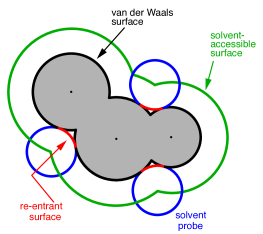
Construction of the cavity surface is a crucial aspect of PCMs, as computed properties are quite sensitive to the details of the cavity construction. Most cavity constructions are based on a union of atom-centered spheres (see Fig. 11.1), but there are yet several different constructions whose nomenclature is occasionally confused in the literature. Simplest and most common is the van der Waals (vdW) surface consisting of a union of atom-centered spheres. The radius for the sphere centered on atom can be written in the form
| (11.4) |
where is the vdW radius for atom , taken for example from the set of vdW
radii published by Bondi.
126
J. Phys. Chem.
(1964),
68,
pp. 441.
Link
Traditionally, the vdW radii
that are extracted from crystallographic data are scaled by a factor
–1.2.
125
J. Am. Chem. Soc.
(1984),
106,
pp. 1945.
Link
,
1194
Chem. Rev.
(1994),
94,
pp. 2027.
Link
,
490
Wiley Interdiscip. Rev.: Comput. Mol. Sci.
(2021),
11,
pp. e1519.
Link
This 20% augmentation is intended to mimic the fact that solvent molecules cannot
approach all the way to the vdW radius of the solute atoms, though it’s not
altogether clear that the same value ought to be optimal in all cases. (The scaling factor defaults to
but can be modified by the user.)
An alternative to scaling
the atomic radii is to add a certain fixed increment to each, representing the
approximate size of a solvent molecule, and leading
to what is known as the solvent accessible surface (SAS).
The choice Å is common for water and represents the approximate
physical size of a water molecule, although values in the range –0.5 Å often
afford better solvation energies.
490
Wiley Interdiscip. Rev.: Comput. Mol. Sci.
(2021),
11,
pp. e1519.
Link
In any case, if a nonzero value of is used, then the scaling factor in
Eq. (11.4) should be set to , since these two parameters
are intended to model the same effect, namely, that a solvent molecule’s finite size prevents it from approaching
all the way to the vdW radii of the solute.
Note from Fig. 11.1 that both the vdW surface and the SAS possess cusps
where the atomic spheres intersect, although these become less pronounced as
the atomic radii are scaled or augmented. These cusps are eliminated in what
is known as the solvent-accessible surface (SES), sometimes called the
Connolly surface or the “molecular surface". The SES uses the surface of the
probe sphere at points where it is simultaneously tangent to two or more atomic
spheres to define elements of a “re-entrant surface” that smoothly connects
the atomic (or “contact”) surface.
659
Mol. Phys.
(2020),
118,
pp. e1644384.
Link
Having chosen a model for the cavity surface, this surface is discretized using
atom-centered Lebedev grids
682
Zh. Vychisl. Mat. Mat. Fix.
(1976),
16,
pp. 293.
Link
of
the same sort that are used to perform the numerical integrations in DFT.
(Discretization of the re-entrant facets of the SES is somewhat more
complicated but similar in spirit.
659
Mol. Phys.
(2020),
118,
pp. e1644384.
Link
) Surface charges
are located at these grid points and the Lebedev quadrature weights can be used
to define the surface area associated with each discretization point.
661
J. Phys. Chem. Lett.
(2010),
1,
pp. 556.
Link
A long-standing (though not well-publicized) problem with the aforementioned
discretization procedure is that it fails to afford continuous potential
energy surfaces as the solute atoms are displaced, because certain surface grid
points may emerge from, or disappear within, the solute cavity, as the atomic
spheres that define the cavity are moved. This undesirable behavior can
inhibit convergence of geometry optimizations and, in certain cases, lead to
very large errors in vibrational frequency calculations.
661
J. Phys. Chem. Lett.
(2010),
1,
pp. 556.
Link
It
is also a fundamental hindrance to molecular dynamics
calculations.
662
J. Chem. Phys.
(2010),
133,
pp. 244111.
Link
Building upon earlier work by York and
Karplus,
1326
J. Phys. Chem. A
(1999),
103,
pp. 11060.
Link
Lange and
Herbert
661
J. Phys. Chem. Lett.
(2010),
1,
pp. 556.
Link
,
662
J. Chem. Phys.
(2010),
133,
pp. 244111.
Link
,
659
Mol. Phys.
(2020),
118,
pp. e1644384.
Link
developed a general scheme
for implementing apparent surface charge PCMs in a manner that affords smooth
potential energy surfaces, even for ab initio molecular dynamics
simulations involving bond breaking.662, 484, 490
Notably, this approach is faithful to the properties of the underlying integral
equation theory on which the PCMs are based, in the sense that the smoothing
procedure does not significantly perturb solvation energies or cavity surface
areas.
661
J. Phys. Chem. Lett.
(2010),
1,
pp. 556.
Link
,
662
J. Chem. Phys.
(2010),
133,
pp. 244111.
Link
The smooth discretization procedure
combines a switching function with Gaussian blurring of the cavity surface
charge density, and is thus known as the “Switching/Gaussian” (SwiG)
implementation of the PCM.
Both single-point energies and analytic energy gradients are available for SwiG-PCMs,
when the solute is described using molecular mechanics or an SCF
(Hartree-Fock or DFT) electronic structure model, except that for the SES
cavity model only single-point energies are available. Analytic Hessians are
available for the C-PCM model only. (As usual, vibrational frequencies for
other models will be computed, if requested, by finite difference of analytic
energy gradients.) Single-point energy calculations using correlated wave
functions can be performed in conjunction with these solvent models, in which
case the correlated wave function calculation will use Hartree-Fock molecular
orbitals that are polarized in the presence of the continuum dielectric solvent
(i.e., there is no post-Hartree–Fock PCM correction). This represents a “zeroth-order”
inclusion of solvent effects that captures the leading-order effect of continuum solvation on
molecular properties. Given the crudeness of the model itself, more consistent inclusion of
post-Hartree–Fock solvation effects is not expected to be important.
490
Wiley Interdiscip. Rev.: Comput. Mol. Sci.
(2021),
11,
pp. e1519.
Link
Researchers who use these PCMs are asked to cite
Refs.
662
J. Chem. Phys.
(2010),
133,
pp. 244111.
Link
and
664
Chem. Phys. Lett.
(2011),
509,
pp. 77.
Link
, which provide the details of
Q-Chem’s implementation, and Ref.
659
Mol. Phys.
(2020),
118,
pp. e1644384.
Link
if the SES is used.
We point the reader in particular to Refs.
662
J. Chem. Phys.
(2010),
133,
pp. 244111.
Link
and
1330
J. Chem. Phys.
(2015),
143,
pp. 204104.
Link
, which
provides an assessment of the discretization errors that can be anticipated
using various PCMs and Lebedev grids; default grid values in Q-Chem were
established based on these tests.
When publishing results based on PCM
calculations, it is essential to specify both the precise model that is used
(see Table 11.3) as well as how the cavity was constructed, and this should be done
without resorting to software-specific keywords, the use of which has significantly muddled the
literature on continuum electrostatics.
243
Acc. Chem. Res.
(2009),
42,
pp. 493.
Link
,
490
Wiley Interdiscip. Rev.: Comput. Mol. Sci.
(2021),
11,
pp. e1519.
Link
As an example of good practice,
the default cavity construction in Q-Chem is a vdW cavity using Bondi atomic radii,
126
J. Phys. Chem.
(1964),
68,
pp. 441.
Link
except that for hydrogen we use the modified radius of 1.1 Å,
following a reassessment that judged Bondi’s original value of 1.2 Å for hydrogen to be too
large.
1040
J. Phys. Chem.
(1996),
100,
pp. 7384.
Link
Each of these radii in Eq. (11.4) is then
scaled by a factor for use in cavity construction.
Radii for main-group elements that were not provided by Bondi are
taken from Ref.
773
J. Phys. Chem. A
(2009),
113,
pp. 5806.
Link
. Absent details such as these,
PCM calculations will be difficult to reproduce in other electronic structure programs.
In vertical excitation or ionization, the solute undergoes a sudden change in
its charge distribution. Various microscopic motions of the solvent have
characteristic times to reach certain polarization response, and fast part of
the solvent response (electrons) can follow such a dynamic process while the
remaining degrees of freedom (nuclei) remain unchanged as in the initial state.
Such splitting of the solvent response gives rise to nonequilibrium solvation.
In the literature, two different approaches have been developed for describing
nonequilibrium solvent effects: the linear response (LR)
approach
157
J. Chem. Phys.
(1999),
110,
pp. 9877.
Link
,
238
J. Chem. Phys.
(2001),
115,
pp. 4708.
Link
and the state-specific (SS)
approach.
1194
Chem. Rev.
(1994),
94,
pp. 2027.
Link
,
158
Int. J. Quantum Chem. Symp.
(1995),
29,
pp. 465.
Link
,
236
J. Phys. Chem. A
(2000),
104,
pp. 10614.
Link
,
531
J. Chem. Phys.
(2006),
125,
pp. 054103.
Link
Both are
implemented in Q-Chem,
1330
J. Chem. Phys.
(2015),
143,
pp. 204104.
Link
,at the SCF level for vertical
ionization and at the corresponding level (CIS, TDDFT or ADC, see
Section 7.11.10) for vertical excitation. A brief introduction to
these methods is given below, and users of the nonequilibrium PCM features are
asked to cite Refs.
1330
J. Chem. Phys.
(2015),
143,
pp. 204104.
Link
and
818
J. Phys. Chem. A
(2015),
119,
pp. 5446.
Link
.
State-specific solvent-field equilibration for long-lived excited states to
compute e.g. emission energies is implemented for the ADC-suite of methods as
described in Section 7.11.10. Users of this equilibrium-solvation
PCM please cite and be referred to Ref.
817
Phys. Chem. Chem. Phys.
(2017),
19,
pp. 1644.
Link
.
The LR approach considers the solvation effects as a coupling between a pair of
transitions, one for solute and the other for solvent. The transition
frequencies when the interaction between the solute and solvent is turned on
may be determined by considering such an interaction as a perturbation. In the
framework of TDDFT, the solvent/solute interaction is given by
518
J. Chem. Phys.
(2001),
114,
pp. 3065.
Link
| (11.5) |
where is the charge density response function of the solvent and is the solute’s transition density. This term accounts for a dynamical correction to the transition energy so that it is related to the response of the solvent to the charge density of the solute oscillating at the solute transition frequency (). Within a PCM, only classical Coulomb interactions are taken into account, and Eq. (11.5) becomes
| (11.6) |
where is PCM solvent response operator for a generic dielectric constant, . The integral of and the potential of the density gives the surface charge density for the solvent polarization.
The state-specific approach takes into account the capability of a part of the solvent degrees of freedom to respond instantaneously to changes in the solute wave function upon excitation. Such an effect is not accounted for in the LR approach. In SS, a generic solvated-solute excited state is obtained as a solution of a nonlinear Schrödinger equation
| (11.7) |
that depends upon the solute’s charge distribution. Here is
the usual Hamiltonian for the solute in vacuum and the reaction field operator
generates the electrostatic potential of the apparent surface
charge density (Section 11.2.3.1), corresponding to
slow and fast polarization response.
The solute is polarized self-consistently with respect to the solvent’s
reaction field. In case of vertical ionization rather than excitation, both the
ionized and non-ionized states can be treated within a ground-state formalism.
For vertical excitations, self-consistent SS models have been developed for
various excited-state methods,
531
J. Chem. Phys.
(2006),
125,
pp. 054103.
Link
,
792
Chem. Sci.
(2011),
2,
pp. 2143.
Link
including both
CIS and TDDFT.
In a linear dielectric medium, the solvent polarization is governed by the
electric susceptibility, , where
is the frequency-dependent permittivity.
In case of very fast vertical transitions, the dielectric response is ruled by
the optical dielectric constant, , where is
the solvent’s index of refraction. In both LR and SS, the fast part of the
solvent’s degrees of freedom is in equilibrium with the solute density change.
Within PCM, the fast solvent polarization charges for the SS excited state
can be obtained by solving the following equation:
236
J. Phys. Chem. A
(2000),
104,
pp. 10614.
Link
| (11.8) |
Here is the discretized fast surface charge. The dielectric constants in the matrices and (Section 11.2.3.1) are replaced with the optical dielectric constant, and is the potential of the solute’s excited state density, . The quantity is the potential of the slow part of the apparent surface charges in the ground state, which are given by
| (11.9) |
For LR-PCM, the solvent polarization is subjected to the first-order changes to the electron density (TDDFT linear density response), and thus Eq. (11.8) becomes
| (11.10) |
The LR approach for CIS/TDDFT excitations and the self-consistent SS
method (using the ground-state SCF) for vertical ionizations are available in
Q-Chem. The self-consistent SS method for vertical excitations is not
available, because this method is problematic in the vicinity of (near-)
degeneracies between excited states, such as in the vicinity of a conical
intersection. The fundamental problem in the SS approach is that each wave
function is an eigenfunction of a different Hamiltonian, since
Eq. (11.7) depend upon the specific state of interest. To avoid the
ordering and the non-orthogonality problems, we compute the vertical
excitation energy using a first-order, perturbative approximation to the SS
approach,
156
J. Chem. Phys.
(2005),
122,
pp. 104513.
Link
,
163
J. Chem. Phys.
(2006),
124,
pp. 124520.
Link
in what we have termed the “ptSS”
method.
818
J. Phys. Chem. A
(2015),
119,
pp. 5446.
Link
The zeroth-order excited-state wave function can be
calculated using various excited-state methods (currently available for CIS and
TDDFT in Q-Chem) with solvent-relaxed molecular orbitals obtained from a
ground-state PCM calculation. As mentioned previously, LR and SS describe
different solvent relaxation features in nonequilibrium solvation. In the
perturbation scheme, we can calculate the LR contribution using the
zeroth-order transition density, in what we have called the “ptLR” approach.
The combination of ptSS and ptLR yields quantitatively good solvatochromatic
shifts in combination with TDDFT but not with the correlated variants of ADC,
for which the pure ptSS approach was shown to be superior.
1330
J. Chem. Phys.
(2015),
143,
pp. 204104.
Link
,
818
J. Phys. Chem. A
(2015),
119,
pp. 5446.
Link
The LR and SS approaches can also be used in the study of photon emission
processes.
532
J. Chem. Phys.
(2007),
127,
pp. 074504.
Link
An emission process can be treated as a vertical
excitation at a stationary point on the excited-state potential surface. The
basic requirement therefore is to prepare the solvent-relaxed geometry for the
excited-state of interest. TDDFT/C-PCM analytic gradients and Hessian are available.
Section 7.3.5 for computational details regarding excited-state geometry optimization with PCM. An emission process is slightly more complicated than the absorption case. Two scenarios are discussed in literature, depending on the lifetime of an excited state in question. In the limiting case of ultra-fast excited state decay, when only fast solvent degrees of freedom are expected to be equilibrated with the excited-state density. In this limit, the emission energy can be computed exactly in the same way as the vertical excitation energy. In this case, excited state geometry optimization should be performed in the nonequilibrium limit. The other limit is that of long-lived excited state, e.g., strongly fluorescent species and phosphorescence. In the long-lived case, excited state geometry optimization should be performed with the solvent equilibrium limit. Thus, the excited state should be computed using an equilibrium LR or SS approach, and the ground state is calculated using nonequilibrium self-consistent SS approach. The latter approach is implemented for the ADC-based methods as described in Section 7.11.10.
For ultrafast processes in solution, such as electron transfer, photo-absorption/emission and photo-ionization,
a continuum model should combine a proper nonequilibrium solvation theory to account for nonequilibrium solute–solvent interactions.
In the traditional treatments, the nonequilibrium electrostatic solvation free energy was derived from the so-called reversible electric work integration along the path linking the initial equilibrium state (eq) and the intermediate nonequilibrium state (neq),
785
J. Chem. Phys.
(1956),
24,
pp. 966.
Link
,
786
J. Chem. Phys.
(1956),
24,
pp. 979.
Link
i.e.,
| (11.11) |
where denotes the total electric potential including both the potential due to the solute charge in vacuum and polarization potential due to the medium.
In order to deal with electron absorption and emission spectra in solution, the numerical expression of nonequilibrium solvation free energy which was established by intuitively collecting a series of energy terms from the interactions of solute charges and polarized charges, has been implemented using TDDFT with PCM model.
236
J. Phys. Chem. A
(2000),
104,
pp. 10614.
Link
,
237
J. Chem. Phys.
(2000),
112,
pp. 2427.
Link
It is easy to verify this numerical form can be achieved through the discretization of analytical expression of nonequilibrium solvation energy by traditional treatments.
721
Int. J. Quantum Chem.
(2015),
115,
pp. 700.
Link
However, there exist a number of doubts on the overestimation of the solvent reorganization energy in ultrafast processes by this reversible electric work method.
115
J. Phys. Chem.
(1990),
94,
pp. 1788.
Link
,
407
J. Phys. Chem. A
(2010),
114,
pp. 2778.
Link
It becomes clear now that there is no possibility to find a reversible pathway between the initial equilibrium state and the intermediate nonequilibrium state. Thus, the integrated electric work can not equal to the change of electrostatic free energy.
721
Int. J. Quantum Chem.
(2015),
115,
pp. 700.
Link
Xiangyuan Li et al.
721
Int. J. Quantum Chem.
(2015),
115,
pp. 700.
Link
,
1304
Phys. Chem. Chem. Phys.
(2012),
14,
pp. 5538.
Link
,
1015
J. Phys. Chem. A
(2013),
117,
pp. 8017.
Link
established the new theory for nonequilibrium solvation by employing the constrained equilibrium principle
using the following pathway
| (11.12) |
where C stands for the constrained equilibrium state which is constructed and mapped to the true nonequilibrium state by introducing the proper external charge which is used to equilibrate the “residual” polarization potential, . In this way the solvent reorganization energy can be derived as
| (11.13) |
Then the nonequilibrium solvation free energy is simply given by
| (11.14) |
For more detailed descriptions of the gain of the external (constraining) charge , or the equivalent constraining external electric field , please refer to the review.
721
Int. J. Quantum Chem.
(2015),
115,
pp. 700.
Link
Within the framework of continuum model, the discretization and numerical solution of Eq. (11.14) is expressed as
113
Phys. Chem. Chem. Phys.
(2017),
19,
pp. 32242.
Link
| (11.15) |
where the subscript denotes the ground ( = 1) or excited ( = 2) electronic state. The value refers to the solute electrostatic potential at the mth tesserae. is the apparent charge for the nonequilibrium state. is the square matrix based on PCM versions (CPCM, IEFPCM, SSVPE, etc.).
The vertical excitation energy for absorption is defined as
| (11.16) |
where stands for total free energy of the solute in solution,
| (11.17) |
is calculated by the self-consistent reaction field (SCRF) method based on equilibrium ground-state reaction field and means ground-state electronic energy of the solute. Based on the equilibrium ground-state reaction field, with a self-consistent state-specific method in the framework of TDDFT, is given by
113
Phys. Chem. Chem. Phys.
(2017),
19,
pp. 32242.
Link
| (11.18) |
is the excitation energy from TDDFT calculation.Alternatively, based on the nonequilibrium excited-state reaction field, is given by
112
Phys. Chem. Chem. Phys.
(2018),
20,
pp. 13178.
Link
| (11.19) |
where represents the th iteration of the nonequilibrium excited-state reaction field at the ground-state geometry of solute. is the excitation energy from TDDFT calculation in the presence of the nonequilibrium excited-state reaction field. stands for the ground-state electronic energy of solute at the th iteration. Clearly, Eq. (11.19) is more physically-meaningful than Eq. (11.18).
Similarly, the vertical excitation energy for emission is given by
112
Phys. Chem. Chem. Phys.
(2018),
20,
pp. 13178.
Link
| (11.20) |
where and represent the free energies of the equilibrium excited state and the nonequilibrium ground state at the excited-state equilibrium geometry, respectively, which can be expressed as
112
Phys. Chem. Chem. Phys.
(2018),
20,
pp. 13178.
Link
| (11.21) |
| (11.22) |
can be directly obtained by TDDFT calculation in the equilibrium excited-state reaction field at the th iteration and is the corresponding ground-state electronic energy of the solute. is the ground-state electronic energy of the solute at the excited-state equilibrium geometry in the presence of the nonequilibrium ground-state reaction field.
The keyword TdNonEq is requested in the $pcm section.
Refs.
721
Int. J. Quantum Chem.
(2015),
115,
pp. 700.
Link
should be cited if constrained equilibrium principle is employed to obtained the vertical absorption/emission energies in solution using the self-consistent state-specific (SS)-PCM/TDDFT method.