12.7 The Explicit Polarization (XPol) Method
12.7.1 Theory
XPol is an approximate, fragment-based molecular orbital method that was developed as a “next-generation” force field [705, 706, 688, 707]. The basic idea of the method is to treat a molecular liquid, solid, or cluster as a collection of fragments, where each fragment is a molecule. Intra-molecular interactions are treated with a self-consistent field method (Hartree-Fock or DFT), but each fragment is embedded in a field of point charges that represent electrostatic interactions with the other fragments. These charges are updated self-consistently by collapsing each fragment’s electron density onto a set of atom-centered point charges, using charge analysis procedures (Mulliken, Löwdin, or CHELPG, for example; see Section 10.2.1). This approach incorporates many-body polarization, at a cost that scales linearly with the number of fragments, but neglects the antisymmetry requirement of the total electronic wavefunction. As a result, intermolecular exchange-repulsion is neglected, as is dispersion since the latter is an electron correlation effect. As such, the XPol treatment of polarization must be augmented with empirical, Lennard–Jones-type intermolecular potentials in order to obtain meaningful optimized geometries, vibrational frequencies or dynamics.
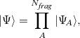
The XPol method is based upon an ansatz in which the supersystem wavefunction is written as a direct product of fragment wavefunctions,
 |
(12.1) |
where  is the number of fragments. We assume here that the fragments are molecules and that covalent bonds remain intact. The fragment wavefunctions are antisymmetric with respect to exchange of electrons within a fragment, but not to exchange between fragments. For closed-shell fragments described by Hartree-Fock theory, the XPol total energy is [688, 689]
![\begin{equation} \label{eq:E_ xpol} E_{\rm XPol} = \sum _ A \left[ 2 \sum _{a} \mathbf{c}_ a^\dagger \left( \mathbf{h}^ A+ \mathbf{J}^ A - \tfrac {1}{2}\mathbf{K}^ A \right) \mathbf{c}_ a^{} +E_{nuc}^ A \right] + E_{embed} . \end{equation}](images/img-1778.png) |
(12.2) |
The term in square brackets is the ordinary Hartree-Fock energy expression for fragment  . Thus,
  is a vector of occupied MO expansion coefficients (in the AO basis) for the occupied MO
  ;
;  consists of the one-electron integrals; and
  and
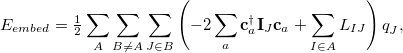
and  are the Coulomb and exchange matrices, respectively, constructed from the density matrix for fragment . The additional terms in Eq. eq:E_xpol,
 |
(12.3) |
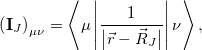
arise from the electrostatic embedding. The matrix  is defined by its AO matrix elements,
 |
(12.4) |
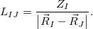
and  is given by
 |
(12.5) |
According to Eqs. eq:E_xpol and eq:E_QMMM, each fragment is embedded in the electrostatic potential arising from a set of point charges,  , on all of the other fragments; the factor of
  in Eq. eq:E_QMMM avoids double-counting. Exchange interactions between fragments are ignored, and the electrostatic interactions between fragments are approximated by interactions between the charge density of one fragment and point charges on the other fragments.
Crucially, the vectors  are constructed within the ALMO ansatz [683], so that MOs for each fragment are represented in terms of only those AOs that are centered on atoms in the same fragment. This choice affords a method whose cost grows linearly with respect to , and where basis set superposition error is excluded by construction. In compact basis sets, the ALMO ansatz excludes inter- fragment charge transfer as well.
The original XPol method of Xie et al. [706, 688, 707] uses Mulliken charges for the embedding charges  in Eq. eq:E_QMMM, though other charge schemes could be envisaged. In non-minimal basis sets, the use of Mulliken charges is beset by severe convergence problems [689], and Q-Chem’s implementation of XPol offers the alternative of using either Löwdin charges or “CHELPG” charges [455], the latter being. derived from the electrostatic potential as discussed in Section 10.2.1. The CHELPG charges are found to be stable and robust, albeit with a somewhat larger computational cost as compared to Mulliken or Löwdin charges [689, 456]. An algorithm to compute CHELPG charges using atom-centered Lebedev grids rather than traditional Cartesian grids is available [457] (see Section 10.2.1), which uses far fewer grid points and thus can significantly improve the performance for the XPol/CHELPG method, where these charges must be iteratively updated.
Researchers who use Q-Chem’s XPol code are asked to cite Refs. Jacobson:2011, and Herbert:2012.
12.7.2 Supplementing XPol with Empirical Potentials
In order to obtain physical results, one must either supplement the XPol energy expression with either empirical intermolecular potentials or else with an ab initio treatment of intermolecular interactions. The latter approach is described in Section 12.9. Here, we describe how to add Lennard-Jones or Buckingham potentials to the XPol energy, using the $xpol_mm and $xpol_params sections described below.
The Lennard-Jones potential is
![\begin{equation} \label{eq:Lennard-Jones} V_{\rm LJ}^{}(R_{ij}) = 4 \epsilon ^{}_{ij} \left[ \left(\frac{\sigma ^{}_{ij}}{R_{ij}}\right)^{\! 12} - \left(\frac{\sigma ^{}_{ij}}{R_{ij}}\right)^{\! 6} \right] \; , \end{equation}](images/img-1793.png) |
(12.6) |
where  represents the distance between atoms
  and
and  . This potential is characterized by two parameters, a well depth
  and a length scale
  . Although quite common, the
  repulsion is unrealistically steep. The Buckingham potential replaces this with an exponential function,
![\begin{equation} \label{eq:Buckingham} V_{\rm Buck}^{}(R_{ij}) = \epsilon ^{}_{ij} \left[ A e^{-B \frac{R_{ij}}{\sigma ^{}_{ij}}} - C \left(\frac{\sigma ^{}_{ij}}{R_{ij}}\right)^{\! 6} \right] \; , \end{equation}](images/img-1797.png) |
(12.7) |
Here, ,  , and
, and  are additional (dimensionless) constants, independent of atom type. In both Eq. eq:Lennard-Jones and Eq. eq:Buckingham, the parameters and
  are determined using the geometric mean of atomic well-depth and length-scale parameters. For example,
 |
(12.8) |
The atomic parameters  and
and  must be specified using a $xpol_mm section in the Q-Chem input file. The format is a molecular mechanics-like specification of atom types and connectivities. All atoms specified in the $molecule section must also be specified in the $xpol_mm section. Each line must contain an atom number, atomic symbol, Cartesian coordinates, integer atom type, and any connectivity data. The $xpol_params section specifies, for each atom type, a value for
  in kcal/mol and a value for
  in Angstroms. A Lennard-Jones potential is used by default; if a Buckingham potential is desired, then the first line of the $xpol_params section should contain the string BUCKINGHAM followed by values for the , , and parameters.
12.7.3 Job Control Variables for XPol
XPol calculations are enabled by setting the $rem variable XPOL to TRUE. These calculations can be used in combination with Hartree-Fock theory and with most density functionals, a notable exception being that XPol is not yet implemented for meta-GGA functionals (Section 4.3.3). Combining XPol with solvation models (Section 11.2) or external charges ($external_charges) is also not available. Analytic gradients are available when Mulliken or Löwdin embedding charges are used, but not yet available for CHELPG embedding charges.
XPOL
Perform a self-consistent XPol calculation.
TYPE:
BOOLEAN
DEFAULT:
FALSE
OPTIONS:
TRUE
Perform an XPol calculation.
FALSE
Do not perform an XPol calculation.
RECOMMENDATION:
NONE
XPOL_CHARGE_TYPE
Controls the type of atom-centered embedding charges for XPol calculations.
TYPE:
STRING
DEFAULT:
QLOWDIN
OPTIONS:
QLOWDIN
Löwdin charges.
QMULLIKEN
Mulliken charges.
QCHELPG
CHELPG charges.
RECOMMENDATION:
Problems with Mulliken charges in extended basis sets can lead to XPol convergence failure. Löwdin charges tend to be more stable, and CHELPG charges are both robust and provide an accurate electrostatic embedding. However, CHELPG charges are more expensive to compute, and analytic energy gradients are not yet available for this choice.
XPOL_MPOL_ORDER
Controls the order of multipole expansion that describes electrostatic interactions.
TYPE:
STRING
DEFAULT:
CHARGES
OPTIONS:
GAS
No electrostatic embedding; monomers are in the gas phase.
CHARGES
Charge embedding.
DENSITY
Density embedding.
RECOMMENDATION:
Should be set to GAS to do a dimer SAPT calculation (see Section 12.8).
XPOL_PRINT
Print level for XPol calculations.
TYPE:
INTEGER
DEFAULT:
1
OPTIONS:

Integer print level
RECOMMENDATION:
Higher values prints more information
XPOL_OMEGA
Controls the range-separation parameter,
, that is used in long-range-corrected DFT.
TYPE:
BOOLEAN
DEFAULT:
FALSE
OPTIONS:
TRUE
Use different
FALSE
Use a single value of
RECOMMENDATION:
If FALSE, the $rem variable OMEGA should be used to specify the single value of
OMEGA/1000, in atomic units.
12.7.4 Examples
XPol on its own is not a useful method (as it neglects all intermolecular interactions except for polarization), so the two examples below demonstrate the use of XPol in conjunction with a Lennard-Jones and a Buckingham potential, respectively.
Example 12.273 An XPol single point calculation on the water dimer using a Lennard-Jones potential.
$molecule
0 1
-- water 1
0 1
O          -1.364553     .041159     .045709
H          -1.822645     .429753    -.713256
H          -1.841519    -.786474     .202107
-- water 2
0 1
O           1.540999     .024567     .107209
H            .566343     .040845     .096235
H           1.761811    -.542709    -.641786
$end

$rem
METHOD           HF
BASIS            3-21G
XPOL             TRUE
XPOL_CHARGE_TYPE QLOWDIN
$end

$xpol_mm
1 O          -1.364553     .041159     .045709 1 2 3
2 H          -1.822645     .429753    -.713256 2 1
3 H          -1.841519    -.786474     .202107 2 1
4 O           1.540999     .024567     .107209 1 5 6
5 H            .566343     .040845     .096235 2 4
6 H           1.761811    -.542709    -.641786 2 4
$end

$xpol_params
1            0.16     3.16
2            0.00     0.00
$end
Example 12.274 An XPol single point calculation on the water dimer using a Buckingham potential.
$molecule
0 1
-- water 1
0 1
O          -1.364553     .041159     .045709
H          -1.822645     .429753    -.713256
H          -1.841519    -.786474     .202107
-- water 2
0 1
O           1.540999     .024567     .107209
H            .566343     .040845     .096235
H           1.761811    -.542709    -.641786
$end

$rem
METHOD           HF
BASIS            3-21G
XPOL             TRUE
XPOL_CHARGE_TYPE QLOWDIN
$end

$xpol_mm
1 O          -1.364553     .041159     .045709 1 2 3
2 H          -1.822645     .429753    -.713256 2 1
3 H          -1.841519    -.786474     .202107 2 1
4 O           1.540999     .024567     .107209 1 5 6
5 H            .566343     .040845     .096235 2 4
6 H           1.761811    -.542709    -.641786 2 4
$end

$xpol_params
BUCKINGHAM   500000.0 12.5 2.25
1            0.16     3.16
2            0.00     0.00
$end