12.8 Symmetry-Adapted Perturbation Theory (SAPT)

12.8.1 Theory

Symmetry-adapted perturbation theory (SAPT) is a theory of intermolecular interactions. When computing intermolecular interaction energies one typically computes the energy of two molecules infinitely separated and in contact, then computes the interaction energy by subtraction. SAPT, in contrast, is a perturbative expression for the interaction energy itself. The various terms in the perturbation series are physically meaningful, and this decomposition of the interaction energy can aid in the interpretation of the results. A brief overview of the theory is given below; for additional technical details, the reader is referred to Jeziorski et al. [708, 690]. Additional context can be found in a pair of more recent review articles [691, 709].

In SAPT, the Hamiltonian for the $\rm A\cdots B$ dimer is written as

$\begin{equation} \label{eq:H_ SAPT} \Hat {H} = \Hat {F}^ A + \Hat {F}^ B + \xi \Hat {W}^ A + \eta \Hat {W}^ B + \zeta \Hat {V} \; , \end{equation}$

(12.9)

where $\Hat {W}^ A$ and $\Hat {W}^ B$ are Møller-Plesset fluctuation operators for fragments $A$ and $B$ , whereas $\hat V$ consists of the intermolecular Coulomb operators. This part of the perturbation is conveniently expressed as

$\begin{equation} \hat{V} = \sum _{i\in A} \sum _{j\in B} \Hat {v}(ij) \end{equation}$

(12.10)

with

$\begin{equation} \label{eq:pairwise_ perturbation} \Hat {v}(ij) = \frac{1}{\bigl |\vec{r}_ i-\vec{r}_ j\bigr |} + \frac{\hat{v}_ A(j)}{N_ A} + \frac{\hat{v}_ B(i)}{N_ B} + \frac{V_0}{N_ A N_ B} \; . \end{equation}$

(12.11)

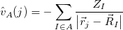
The quantity $V_0$ is the nuclear interaction energy between the two fragments and

$\begin{equation} \label{va_ sapt} \Hat {v}_ A(j) = -\sum _{I\in A} \frac{Z_ I}{\bigl |\vec{r}_ j - \vec{R}_ I\bigr |} \end{equation}$

(12.12)

describes the interaction of electron $j \in B$ with nucleus $I\in A$ .

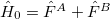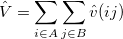
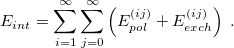
Starting from a zeroth-order Hamiltonian $\Hat {H}_0 = \Hat {F}^ A + \Hat {F}^ B$ and zeroth-order wavefunctions that are direct products of monomer wavefunctions, $|\Psi _0 \rangle = |\Psi _ A\rangle |\Psi _ B\rangle$ , the SAPT approach is based on a symmetrized Rayleigh-Schrödinger perturbation expansion [708, 690] with respect to the perturbation parameters $\xi$ , $\eta$ , and $\zeta$ in Eq. eq:H_SAPT. The resulting interaction energy can be expressed as[708, 690]

$\begin{equation} \label{eq:triple_ pert} E_{int} = \sum _{i=1}^\infty \sum _{j=0}^\infty \left(E^{(ij)}_{pol} + E^{(ij)}_{exch}\right) \; . \end{equation}$

(12.13)

Because it makes no sense to treat $\Hat {W}^ A$ and $\Hat {W}^ B$ at different orders of perturbation theory, there are only two indices in this expansion: $j$ for the monomer fluctuations potentials and $i$ for the intermolecular perturbation. The terms $E^{(ij)}_{pol}$ are known collectively as the polarization expansion, and these are precisely the same terms that would appear in ordinary Rayleigh-Schrödinger perturbation theory, which is valid when the monomers are well-separated. The polarization expansion contains electrostatic, induction and dispersion interactions, but in the symmetrized Rayleigh-Schrödinger expansion, each term $E^{(ij)}_{pol}$ has a corresponding exchange term, $E^{(ij)}_{exch}$ , that arises from an antisymmetrizer $\Hat {\cal A}_{AB}$ that is introduced in order to project away the Pauli-forbidden components of the interaction energy that would otherwise appear [690].

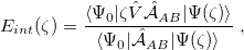
The version of SAPT that is implemented in Q-Chem assumes that $\xi =\eta =0$ , an approach that is usually called SAPT0 [709]. Within the SAPT0 formalism, the interaction energy is formally expressed by the following symmetrized Rayleigh-Schrödinger expansion [708, 690]:

$\begin{equation} \label{eq:E(SRS)} E_{int}(\zeta ) = \frac{ \langle \Psi _0|\zeta \Hat {V}\Hat {\cal A}_{AB}|\Psi (\zeta )\rangle }{ \langle \Psi _0|\Hat {\cal A}_{AB}|\Psi (\zeta )\rangle } \; , \end{equation}$

(12.14)

The antisymmetrizer $\Hat {\cal A}_{AB}$ in this expression can be written as

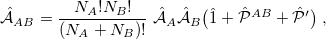$\begin{equation} \label{eq:AB_ antisymmetrizer} \Hat {\cal A}_{AB} = \frac{N_ A! N_ B!}{(N_ A+N_ B)!} \; \Hat {\cal A}_ A \Hat {\cal A}_ B\bigl ( \Hat {1} + \Hat {\cal P}^{AB} + \Hat {\cal P}’ \bigr ) \; , \end{equation}$

(12.15)

where $\Hat {\cal A}_ A$ and $\Hat {\cal A}_ B$ are antisymmetrizers for the two monomers and $\Hat {\cal P}^{AB}$ is a sum of all one-electron exchange operators between the two monomers. The operator $\Hat {\cal P}’$ in Eq. eq:AB_antisymmetrizer denotes all of the three-electron and higher-order exchanges. This operator is neglected in what is known as the “single-exchange” approximation [708, 690], which is expected to be quite accurate at typical van der Waals and larger intermolecular separations, but sometimes breaks down at smaller intermolecular separations [710].

Only terms up to $\zeta =2$ in Eq. eq:E(SRS)—that is, second order in the intermolecular interaction—have been implemented in Q-Chem. It is common to relabel these low-order terms in the following way [cf. Eq. eq:triple_pert]:

$\begin{equation} \label{eq:SAPT_ interaction} E_{int}^{\rm SAPT0} = E^{(1)}_{elst} + E^{(1)}_{exch} + E_{pol}^{(2)} + E_{exch}^{(2)} \; . \end{equation}$

(12.16)

The electrostatic part of the first-order energy correction is denoted $E^{(1)}_{elst}$ and represents the Coulomb interaction between the two monomer electron densities [690]. The quantity $E^{(1)}_{exch}$ is the corresponding first-order (i.e., Hartree-Fock) exchange correction. Explicit formulas for these corrections can be found in Ref. Jeziorski:1993. 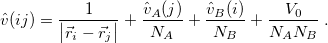The second-order term from the polarization expansion, denoted $E_{pol}^{(2)}$ in Eq. eq:SAPT_interaction, consists of a dispersion contribution (which arises for the first time at second order) as well as a second-order correction for induction. The latter can be written

$\begin{equation} \label{eq:E(2)_ ind} E_{ind}^{(2)} = E_{ind}^{(2)}(A \leftarrow B) + E_{ind}^{(2)}(B \leftarrow A) \; , \end{equation}$

(12.17)

where the notation $A \leftarrow B$ , for example, indicates that the frozen charge density of $B$ polarizes the density of $A$ . In detail,

$\begin{equation} \label{eq:E(2)_ ind_ A<-B} E_{ind}^{(2)}(A \leftarrow B) = 2 \sum _{ar} t_{ar} (w_ B^{})_{ra} \end{equation}$

(12.18)

where

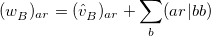$\begin{equation} \label{eq:w_ B} (w_ B^{})_{ar} = (\hat{v}_ B^{})_{ar} + \sum _ b (ar|bb) \end{equation}$

(12.19)

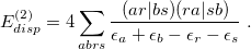
and 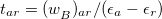$t_{ar} = (w_ B^{})_{ar}/(\epsilon _ a - \epsilon _ r)$ . The second term in Eq. eq:E(2)_ind, in which $A$ polarizes $B$ , is obtained by interchanging labels [689]. The second-order dispersion correction has a form reminiscent of the MP2 correlation energy:

$\begin{equation} \label{eq:E(2)_ disp} E_{disp}^{(2)} = 4 \sum _{abrs} \frac{ (ar|bs) (ra|sb)}{\epsilon _ a + \epsilon _ b - \epsilon _ r - \epsilon _ s} \; . \end{equation}$

(12.20)

The induction and dispersion corrections both have accompanying exchange corrections (exchange-induction and exchange-dispersion) [708, 690].

The similarity between Eq. eq:E(2)_disp and the MP2 correlation energy means that SAPT jobs, like MP2 calculations, can be greatly accelerated using resolution-of-identity (RI) techniques, and an RI version of SAPT is available in Q-Chem. To use it, one must specify an auxiliary basis set. The same ones used for RI-MP2 work equally well for RI-SAPT, but one should always select the auxiliary basis set that is tailored for use with the primary basis of interest, as in the RI-MP2 examples in Section 5.5.1.

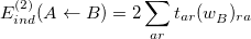
It is common to replace $E_{ind}^{(2)}$ and $E_{exch\text {-}ind}^{(2)}$ in Eq. eq:SAPT_interaction with their “response” ( $resp$ ) analogues, which are the infinite-order correction for polarization arising from a frozen partner density [708, 690]. Operationally, this substitution involves replacing the second-order induction amplitudes, $t_{ar}$ in Eq. eq:E(2)_ind_A<-B, with amplitudes obtained from solution of the coupled-perturbed Hartree-Fock equations [442]. (The perturbation is simply the electrostatic potential of the other monomer.) In addition, it is common to correct the SAPT0 binding energy for higher-order polarization effects by adding a correction term of the form [690, 709]

$\begin{equation} \label{eq:delta_ hf} \delta E_{int}^{\rm HF} = E_{int}^{\rm HF} - \Bigl ( E_{elst}^{(1)} + E_{exch}^{(1)} + E_{ind,resp}^{(2)} + E_{exch\text {-}ind,resp}^{(2)}\Bigr ) \end{equation}$

(12.21)

to the interaction energy. Here, $E_{int}^{\rm HF}$ is the counterpoise-corrected Hartree-Fock binding energy for $\rm A\cdots B$ . Both the response corrections and the $\delta E^{\rm HF}_{\rm int}$ correction have been implemented as options in Q-Chem’s implementation of SAPT.

It is tempting to replace Hartree-Fock MOs and eigenvalues in the SAPT0 formulas with their Kohn-Sham counterparts, as a low-cost means of introducing monomer electron correlation. The resulting procedure is known as SAPT(KS) [711], and does offer an improvement on SAPT0 for some strongly hydrogen-bonded systems [456]. Unfortunately, SAPT(KS) results are generally in poor agreement with benchmark dispersion energies [456], owing to incorrect asymptotic behavior of approximate exchange-correlation potentials [712]. The dispersion energies can be greatly improved through the use of long-range corrected (LRC) functionals in which the range-separation parameter, $\omega$ , is “tuned” so as to satisfy the condition $\epsilon _{\rm HOMO}^{} = -\mbox{IP}$ , where $\epsilon _{\rm HOMO}^{}$ is the HOMO energy and “IP" represents the ionization potential [713]. Monomer-specific values of $\omega$ , tuned using the individual monomer IPs, substantially improve SAPT(KS) dispersion energies, though the results are still not of benchmark quality [713]. Other components of the interaction energy, however, can be described quite accurately SAPT(KS) in conjunction with a tuned version of LRC- $\omega$ PBE [713]. Use of monomer-specific $\omega$ values is controlled by the variable XPOL_OMEGA in the $rem section, and individual values are entered via an $lrc_omega input section.

Finally, some discussion of basis sets is warranted. Typically, SAPT calculations are performed in the so-called dimer-centered basis set (DCBS) [714], which means that the combined $A + B$ basis set is used to calculate the zeroth-order wavefunctions for both $A$ and $B$ . This leads to the unusual situation that there are more MOs than basis functions: one set of occupied and virtual MOs for each monomer, both expanded in the same (dimer) AO basis. As an alternative to the DCBS, one might calculate $|\Psi _{\! A}\rangle$ using only $A$ ’s basis functions (similarly for $B$ ), in which case the SAPT calculation is said to employ the monomer-centered basis set (MCBS) [714]. However, MCBS results are generally of poorer quality. As an efficient alternative to the DCBS, Jacobson and Herbert [689] introduced a projected (“proj”) basis set, borrowing an idea from dual-basis MP2 calculations [197]. In this approach, the SCF iterations are performed in the MCBS but then Fock matrices for fragments $A$ and $B$ are constructed in the dimer ( $A+B$ ) basis set and “pseudo-canonicalized", meaning that the occupied-occupied and virtual-virtual blocks of these matrices are diagonalized. This procedure does not mix occupied and virtual orbitals, and thus leaves the fragment densities and and zeroth-order fragment energies unchanged. However, it does provide a larger set of virtual orbitals that extend over the partner fragment. This larger virtual space is then used to evaluate the perturbative corrections. All three of these basis options (MCBS, DCBS, and projected basis) are available in Q-Chem.

12.8.2 Job Control for SAPT Calculations

Q-Chem’s implementation of SAPT0 was designed from the start as a correction for XPol calculations, a functionality that is described in Section 12.9. As such, a SAPT calculation is requested by setting both of the $rem variable SAPT and XPOL to TRUE. (Alternatively, one may set RISAPT=TRUE to use the RI version of SAPT.) If one wishes to perform a traditional SAPT calculation based on gas-phase SCF monomer wavefunctions rather than XPol monomer wavefunctions, then the $rem variable XPOL_MPOL_ORDER should be set to GAS.

SAPT energy components are printed separately at the end of a SAPT job. If EXCHANGE = HF, then the calculation corresponds to SAPT0, whereas a SAPT(KS) calculation is requested by specifying the desired density functional. [Note that meta-GGAs are not yet available for SAPT(KS) calculations in Q-Chem.] At present, only single-point energies for closed-shell (restricted) calculations are possible. Frozen orbitals are also unavailable.

Researchers who use Q-Chem’s SAPT code are asked to cite Refs. Jacobson:2011 and Herbert:2012.

SAPT

Requests a SAPT calculation.

TYPE:

BOOLEAN

DEFAULT:

FALSE

OPTIONS:

TRUE

Run a SAPT calculation.

FALSE

Do not run SAPT.

RECOMMENDATION:

If SAPT is set to TRUE, one should also specify XPOL=TRUE and XPOL_MPOL_ORDER=GAS.

RISAPT

Requests an RI-SAPT calculation

TYPE:

BOOLEAN

DEFAULT:

FALSE

OPTIONS:

TRUE

Compute four-index integrals using the RI approximation.

FALSE

Do not use RI.

RECOMMENDATION:

Set to TRUE if an appropriate auxiliary basis set is available, as RI-SAPT is much faster and affords negligible errors (as compared to ordinary SAPT) if the auxiliary basis set is matched to the primary basis set. (The former must be specified using AUX_BASIS.)

SAPT_ORDER

Selects the order in perturbation theory for a SAPT calculation.

TYPE:

STRING

DEFAULT:

SAPT2

OPTIONS:

SAPT1

First order SAPT.

SAPT2

Second order SAPT.

ELST

First-order Rayleigh-Schrödinger perturbation theory.

RSPT

Second-order Rayleigh-Schrödinger perturbation theory.

RECOMMENDATION:

SAPT2 is the most meaningful.

SAPT_EXCHANGE

Selects the type of first-order exchange that is used in a SAPT calculation.

TYPE:

STRING

DEFAULT:

S_SQUARED

OPTIONS:

S_SQUARED

Compute first order exchange in the single-exchange (“ $S^2$ ") approximation.

S_INVERSE

Compute the exact first order exchange.

RECOMMENDATION:

The single-exchange approximation is expected to be adequate except possibly at very short intermolecular distances, and is somewhat faster to compute.

SAPT_BASIS

Controls the MO basis used for SAPT corrections.

TYPE:

STRING

DEFAULT:

MONOMER

OPTIONS:

MONOMER

Monomer-centered basis set (MCBS).

DIMER

Dimer-centered basis set (DCBS).

PROJECTED

Projected basis set.

RECOMMENDATION:

The DCBS is more costly than the MCBS and can only be used with XPOL_MPOL_ORDER=GAS (i.e., it is not available for use with XPol). The PROJECTED choice is an efficient compromise that is available for use with XPol.

SAPT_CPHF

Requests that the second-order corrections $E_{ind}^{(2)}$ and $E_{exch\text {-}ind}^{(2)}$ be replaced by their infinite-order “response” analogues, $E_{ind,resp}^{(2)}$ and $E_{exch\text {-}ind,resp}^{(2)}$ .

TYPE:

BOOLEAN

DEFAULT:

FALSE

OPTIONS:

TRUE

Evaluate the response corrections and use $E_{ind,resp}^{(2)}$ and $E_{exch\text {-}ind,resp}^{(2)}$

FALSE

Omit these corrections and use $E_{ind}^{(2)}$ and $E_{exch\text {-}ind}^{(2)}$ .

RECOMMENDATION:

Computing the response corrections requires solving CPHF equations for pair of monomers, which is somewhat expensive but may improve the accuracy when the monomers are polar.

SAPT_DSCF

Request the $\delta E_{int}^{\rm HF}$ correction

TYPE:

BOOLEAN

DEFAULT:

FALSE

OPTIONS:

TRUE

Evaluate this correction.

FALSE

Omit this correction.

RECOMMENDATION:

Evaluating the $\delta E_{int}^{\rm HF}$ correction requires an SCF calculation on the entire (super)system. This corrections effectively yields a “Hartree-Fock plus dispersion” estimate of the interaction energy.

SAPT_PRINT

Controls level of printing in SAPT.

TYPE:

INTEGER

DEFAULT:

1

OPTIONS:

$N$

Integer print level

RECOMMENDATION:

Larger values generate additional output.

SAPT_DISP_CORR

Request an empirical dispersion potential instead of calculating $E_{disp}^{(2)}$ and $E_{exch\text {-}disp}^{(2)}$ directly

TYPE:

BOOLEAN

DEFAULT:

FALSE

OPTIONS:

TRUE

Use a dispersion force field.

FALSE

calculate $E_{disp}^{(2)}$ and $E_{exch\text {-}disp}^{(2)}$ .

RECOMMENDATION:

Using dispersion potentials reduces the scaling from ${O}(N^5)$ to ${O}(N^3)$ with respect to monomer size.

SAPT_DISP_VERSION

Controls which dispersion potential is used for SAPT

TYPE:

INTEGER

DEFAULT:

3

OPTIONS:

1

Use the “first generation” (+D1) dispersion potentials from Hesselmann [715, 693].

2

Use the “second generation” (+D2) dispersion potentials from Podeszwa. [716, 694].

3

Use the “third generation” (+D3) dispersion potentials from Lao [695].

RECOMMENDATION:

Use +D3. Whereas +D1 was fit to reproduce binding energies, the +D2 and +D3 potentials were fit directly to dispersion energies $E_{disp}^{(2)}+E_{exch\text {-}disp}^{(2)}$ computed at the SAPT(DFT) and SAPT2+(3) levels, and performs well for both total binding energies as well as individual energy components [694, 695]. In developing +D3, the training set was expanded to eliminate outliers involving $\pi$ stacking [695].

Example 12.275 Example showing a SAPT0 calculation using the RI approximation in a DCBS.

$rem
BASIS           AUG-CC-PVDZ
AUX_BASIS       RIMP2-AUG-CC-PVDZ
METHOD          HF
RISAPT          TRUE
XPOL            TRUE
XPOL_MPOL_ORDER GAS   ! gas-phase monomer wave functions
SAPT_BASIS      DIMER
SYM_IGNORE      TRUE
$end

$molecule
0 1
-- formamide
0 1
C -2.018649  0.052883 0.000000
O -1.452200  1.143634 0.000000
N -1.407770 -1.142484 0.000000
H -1.964596 -1.977036 0.000000
H -0.387244 -1.207782 0.000000
H -3.117061 -0.013701 0.000000
-- formamide
0 1
C 2.018649 -0.052883 0.000000
O 1.452200 -1.143634 0.000000
N 1.407770  1.142484 0.000000
H 1.964596  1.977036 0.000000
H 0.387244  1.207782 0.000000
H 3.117061  0.013701 0.000000
$end

TRUE	Compute four-index integrals using the RI approximation.
FALSE	Do not use RI.

SAPT1	First order SAPT.
SAPT2	Second order SAPT.
ELST	First-order Rayleigh-Schrödinger perturbation theory.
RSPT	Second-order Rayleigh-Schrödinger perturbation theory.

S_SQUARED	Compute first order exchange in the single-exchange (“ $S^2$ ") approximation.
S_INVERSE	Compute the exact first order exchange.

MONOMER	Monomer-centered basis set (MCBS).
DIMER	Dimer-centered basis set (DCBS).
PROJECTED	Projected basis set.

TRUE	Evaluate the response corrections and use $E_{ind,resp}^{(2)}$ and $E_{exch\text {-}ind,resp}^{(2)}$
FALSE	Omit these corrections and use $E_{ind}^{(2)}$ and $E_{exch\text {-}ind}^{(2)}$ .

TRUE	Use a dispersion force field.
FALSE	calculate $E_{disp}^{(2)}$ and $E_{exch\text {-}disp}^{(2)}$ .

1	Use the “first generation” (+D1) dispersion potentials from Hesselmann [715, 693].
2	Use the “second generation” (+D2) dispersion potentials from Podeszwa. [716, 694].
3	Use the “third generation” (+D3) dispersion potentials from Lao [695].