11.2 Chemical Solvent Models

Ab initio quantum chemistry makes possible the study of gas-phase molecular properties from first principles. In liquid solution, however, these properties may change significantly, especially in polar solvents. Although it is possible to model solvation effects by including explicit solvent molecules in the quantum-chemical calculation (e.g. a super-molecular cluster calculation, averaged over different configurations of the molecules in the first solvation shell), such calculations are very computationally demanding. Furthermore, cluster calculations typically do not afford accurate solvation energies, owing to the importance of long-range electrostatic interactions. Accurate prediction of solvation free energies is, however, crucial for modeling of chemical reactions and ligand/receptor interactions in solution.

Q-Chem contains several different implicit solvent models, which differ greatly in their level of sophistication and realism. These are generally known as self-consistent reaction field (SCRF) models, because the continuum solvent establishes a reaction field (i.e., additional terms in the solute Hamiltonian) that depends upon the solute electron density, and must therefore be updated self-consistently during the iterative convergence of the wavefunction. The simplest and oldest of these models that is available in Q-Chem is the Kirkwood-Onsager model [580, 581, 582], in which the solute molecule is placed inside of a spherical cavity and its electrostatic potential is represented in terms of a single-center multipole expansion. More sophisticated models, which use a molecule-shaped cavity and the full molecular electrostatic potential, include the conductor-like screening model (COSMO) [583] and the closely-related conductor-like PCM (C-PCM) [584, 585, 586], along with the “surface and simulation of volume polarization for electrostatics” [SS(V)PE] model [587]. The latter is also known as the “integral equation formalism” (IEF-PCM) [588, 589].

The C-PCM and IEF-PCM/SS(V)PE are examples of what are called “apparent surface charge” SCRF models, although the term polarizable continuum models (PCMs), as popularized by Tomasi and co-workers [590], is now used almost universally to refer to this class of solvation models. Q-Chem employs a Switching/Gaussian or “SWIG” implementation of these PCMs [591, 592, 593, 594]. This approach resolves a long-standing—though little-publicized—problem with standard PCMs, namely, that the boundary-element methods used to discretize the solute/continuum interface may lead to discontinuities in the potential energy surface for the solute molecule. These discontinuities inhibit convergence of geometry optimizations, introduce serious artifacts in vibrational frequency calculations, and make ab initio molecular dynamics calculations virtually impossible [591, 592]. In contrast, Q-Chem’s SWIG PCMs afford potential energy surfaces that are rigorously continuous and smooth. Unlike earlier attempts to obtain smooth PCMs, the SWIG approach largely preserves the properties of the underlying integral-equation solvent models, so that solvation energies and molecular surface areas are hardly affected by the smoothing procedure.

Other solvent models available in Q-Chem include the “Langevin dipoles” model [595, 596] as well as versions 8 and 12 of the SM $x$ models developed at the University of Minnesota [597, 598]. SM8 and SM12 are based upon the generalized Born method for electrostatics, augmented with atomic surface tensions intended to capture non-electrostatic effects (cavitation, dispersion, exchange repulsion, and changes in solvent structure). Empirical corrections of this sort are also available for the PCMs mentioned above, but within SM8 and SM12 these parameters have been optimized to reproduce experimental solvation energies.

Model	Cavity		Non-	Supported	Derivatives
	Construction	Discretization	Electrostatic	Basis	Available?
			Terms?	Sets
Kirkwood-Onsager	spherical	point charges	no	all	none
Langevin Dipoles	atomic spheres	dipoles in	no	all	none
	(user-definable)	3-d space
C-PCM	atomic spheres	point charges or	user-	all	1st and
	(user-definable)	smooth Gaussians	specified		2nd
SS(V)PE/	atomic spheres	point charges or	user-	all	1st
IEF-PCM	(user-definable)	smooth Gaussians	specified
COSMO	predefined	point charges	none	all	1st and
	atomic spheres				2nd
Isodensity SS(V)PE	isodensity contour	point charges	none	all	none
SM8	predefined	generalized	automatic	6-31G*	1st
	atomic spheres	Born		6-31+G*
				6-31+G**
SM12	predefined	generalized	automatic	all	none
	atomic spheres	Born

Table 11.1: Summary of implicit solvation models available in Q-Chem, indicating how the solute cavity is constructed and discretized, whether non-electrostatic terms are (or can be) included, which basis sets are available for use with each model, and whether analytic first and second derivatives are available for optimizations and frequency calculations.

Table 11.1 summarizes the implicit solvent models that are available in Q-Chem. Solvent models are invoked via the SOLVENT_METHOD keyword, as shown below. Additional details about each particular solvent model can be found in the sections that follow, and Table 11.1 provides a summary of the implicit solvent models that are available in Q-Chem. In general, these methods are available for any SCF level of electronic structure theory, though in the case of SM8 only certain basis sets are supported. Post-Hartree–Fock calculations can be performed by first running an SCF + PCM job, in which case the correlated wavefunction will employ MOs and Hartree-Fock energy levels that are polarized by the solvent. Note that the job-control format for specifying implicit solvent models changed significantly starting in Q-Chem version 4.2.1. This change was made in an attempt to simply and unify the input notation for a large number of different models.

SOLVENT_METHOD

Sets the preferred solvent method.

TYPE:

STRING

DEFAULT:

0

OPTIONS:

0

Do not use a solvation model.

ONSAGER

Use the Kirkwood-Onsager model (Section 11.2.1).

PCM

Use an apparent surface charge, polarizable continuum model

(Section 11.2.2).

ISOSVP

Use the iso-density implementation of the SS(V)PE model

(Section 11.2.5).

COSMO

Use COSMO (similar to C-PCM but with an outlying charge

correction [599, 600]; see Section 11.2.6).

SM8

Use version 8 of the Cramer-Truhlar SM $x$ model (Section 11.2.7.1).

SM12

Use version 12 of the SM $x$ model (Section 11.2.7.2).

CHEM_SOL

Use the Langevin Dipoles model (Section 11.2.8).

RECOMMENDATION:

Consult the literature. PCM is a collective name for a family of models and additional input options may be required in this case, in order to fully specify the model. (See Section 11.2.2.) Several versions of SM12 are available as well, as discussed in Section 11.2.7.2.

Before going into detail about each of these models, a few potential points of confusion warrant mention, with regards to nomenclature. First, “PCM” refers to a family of models that includes C-PCM and SS(V)PE/IEF-PCM (the latter two being completely equivalent [589]). One or the other of these models can be selected by additional job control variables in a $pcm input section, as described in Section 11.2.2. COSMO is very similar to C-PCM but includes a correction for that part of the solute’s electron density that penetrates beyond the cavity (the so-called “outlying charge”) [599, 600]. This is discussed in Section 11.2.6.

Two implementations of the SS(V)PE model are also available. The PCM implementation (which is requested by setting SOLVENT_METHOD = PCM) uses a solute cavity constructed from atom-centered spheres, as with most other PCMs. On the other hand, setting SOLVENT_METHOD = ISOSVP requests an SS(V)PE calculation in which the solute cavity is defined by an isocontour of the solute’s own electron density, as advocated by Chipman [587, 601, 602]. This is an appealing, one-parameter cavity construction, although it is unclear that this construction alone is superior in its accuracy to carefully-parameterized atomic radii [603], at least not without additional, non-electrostatic terms included [604, 605] that are unfortunately not yet available in Q-Chem’s implementation of the isodensity version of SS(V)PE. Moreover, analytic energy gradients are not available for the isodensity cavity construction, whereas they are available when the cavity is constructed from atom-centered spheres. One additional subtlety, which is discussed in detail in Ref. [593], is the fact that the PCM implementation of the equation for the SS(V)PE surface charges [Eq. eq:Kq=Rv] uses an asymmetric $\mathbf{K}$ matrix. In contrast, Chipman’s isodensity implementation uses a symmetrized $\mathbf{K}$ matrix. Although the symmetrized version is somewhat more computationally efficient when the number of surface charges is large, the asymmetric version is better justified, theoretically [593]. (This admittedly technical point is clarified in Section 11.2.2 and in particular in Table 11.2.)

Regarding the accuracy of these models for solvation free energies ( $\Delta G_{298}$ ), SM8 achieves sub-kcal/mol accuracy for neutral molecules, based on comparison to a large database of experimental values, although average errors for ions are more like 4 kcal/mol [606]. To achieve comparable accuracy with IEF-PCM/SS(V)PE, non-electrostatic terms must be included [607, 604, 605]. The SM12 model does not improve upon SM8 in any statistical sense [598], but does lift one important restriction on the level of electronic structure that can be combined with these models. Specifically, the Generalized Born model used in SM8 is based on a variant of Mulliken-style atomic charges, and is therefore parameterized only for a few small basis sets, e.g., 6-31G*. SM12, on the other hand, uses a variety of charge schemes that are stable with respect to basis-set expansion, and can therefore be combined with any level of electronic structure theory for the solute. Quantitative fluid-phase thermodynamics can also be obtained using Klamt’s COSMO-RS approach [608, 609], where RS stands for “real solvent”. The COSMO-RS approach is not included in Q-Chem and requires the COSMOtherm program, which is licensed separately through COSMOlogic [610], but Q-Chem can write the input files that are need by COSMOtherm.

The following sections provide more details regarding theory and job control for the various implicit solvent models that are available in Q-Chem. In addition, recent review articles are available for PCM methods [590], SM $x$ [606], and COSMO [611]. Formal relationships between various PCMs have been discussed in Refs. [601, 593].

11.2.1 Kirkwood-Onsager Model

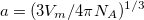
The simplest implicit solvation model available in Q-Chem is the Kirkwood-Onsager model [580, 581, 582], wherein the solute is placed inside of a spherical cavity that is surrounded by a homogeneous dielectric medium. This model is characterized by two parameters: the cavity radius, $a$ , and the solvent dielectric constant, $\varepsilon$ . The former is typically calculated according to

$\begin{equation} \label{eq1000} a = (3V_ m / 4\pi N_ A)^{1/3} \end{equation}$

(11.1)

where $V_ m$ is the solute’s molar volume, usually obtained from experiment (molecular weight or density [612]), and $N_ A$ is Avogadro’s number. It is also common to add 0.5 to the value of $a$ in Eq. (11.1) in order to account for the first solvation shell [613]. Alternatively, $a$ is sometimes selected as the maximum distance between the solute center of mass and the solute atoms, plus the relevant van der Waals radii. A third option is to set $2a$ (the cavity diameter) equal to the largest solute–solvent internuclear distance, plus the the van der Waals radii of the relevant atoms. Unfortunately, solvation energies are typically quite sensitive to the choice of $a$ (and to the construction of the solute cavity, more generally).

Unlike older versions of the Kirkwood-Onsager model, in which the solute’s electron distribution was described entirely in terms of its dipole moment, Q-Chem’s version can use multipoles of arbitrarily high order, including the Born (monopole) term [614] for charged solutes, in order to describe the solute’s electrostatic potential. The solute–continuum electrostatic interaction energy is then computed using analytic expressions for the interaction of the point multipoles with a dielectric continuum.

Energies and analytic gradients for the Kirkwood-Onsager solvent model are available for Hartree-Fock, DFT, and CCSD calculations. It is often advisable to perform a gas-phase calculation of the solute molecule first, which can serve as the initial guess for a subsequent Kirkwood-Onsager implicit solvent calculation.

The Kirkwood-Onsager SCRF is requested by setting SOLVENT_METHOD = ONSAGER in the $rem section (along with normal job control variables for an energy or gradient calculation), and furthermore specifying several additional options in a $solvent input section, as described below. Of these, the keyword CavityRadius is required. The $rem variable CC_SAVEAMPL may save some time for CCSD calculations using the Kirkwood-Onsager model.

NOTE: The following three job control variables belong only in the $solvent section. Do not place them in the $rem section. As with other parts of the Q-Chem input file, this input section is not case-sensitive.

CavityRadius

Sets the radius of the spherical solute cavity.

INPUT SECTION: $solvent
TYPE:

FLOAT

DEFAULT:

No default.

OPTIONS:

$a$

Desired cavity radius, in ngstroms.

RECOMMENDATION:

Use Eq. eq1000.

Dielectric

Sets the dielectric constant of the solvent continuum.

INPUT SECTION: $solvent
TYPE:

FLOAT

DEFAULT:

78.39

OPTIONS:

$\varepsilon$

Use a (dimensionless) value of $\varepsilon$ .

RECOMMENDATION:

As per required solvent; the default corresponds to water at 25 $^\circ$ C.

MultipoleOrder

Determines the order to which the multipole expansion of the solute charge density is carried out.

INPUT SECTION: $solvent
TYPE:

INTEGER

DEFAULT:

15

OPTIONS:

$\ell$

Include up to $\ell$ th order multipoles.

RECOMMENDATION:

Use the default. The multipole expansion is usually converged by order $\ell$ = 15.

Example 11.239 Onsager model applied at the Hartree-Fock level to H $_2$ O in acetonitrile

$molecule
0 1
O       0.00000000     0.00000000     0.11722303
H      -0.75908339     0.00000000    -0.46889211
H       0.75908339     0.00000000    -0.46889211
$end

$rem
method            HF
basis             6-31g**
solvent_method    Onsager
$end

$solvent
CavityRadius      1.8    !   1.8 Angstrom Solute Radius
Dielectric        35.9   !   Acetonitrile
MultipoleOrder    15     !   this is the default value
$end

Example 11.240 CCSD/Onsager calculation applied to 1,2-dichloroethane molecule

$comment
1,2-dichloroethane GAUCHE Conformation
$end

$molecule
0 1
C     0.6541334418569877  -0.3817051480045552   0.8808840579322241
C    -0.6541334418569877   0.3817051480045552   0.8808840579322241
Cl    1.7322599856434779   0.0877596094659600  -0.4630557359272908
H     1.1862455146007043  -0.1665749506296433   1.7960750032785453
H     0.4889356972641761  -1.4444403797631731   0.8058465784063975
Cl   -1.7322599856434779  -0.0877596094659600  -0.4630557359272908
H    -1.1862455146007043   0.1665749506296433   1.7960750032785453
H    -0.4889356972641761   1.4444403797631731   0.8058465784063975
$end

$rem
METHOD           CCSD
BASIS            6-31g**
N_FROZEN_CORE    FC
CC_SAVEAMPL      1         ! Save the CC amplitudes on disk
SOLVENT_METHOD   ONSAGER
$end

$solvent
CavityRadius     3.65  !  in Angstroms
Dielectric       8.93  !  methylene chloride
$end

Example 11.241 Kirkwood-Onsager SCRF applied to hydrogen fluoride in water, performing a gas-phase calculation first.

$molecule
0 1
  H       0.000000     0.000000    -0.862674
  F       0.000000     0.000000     0.043813
$end

$rem
METHOD          HF      
BASIS           6-31G*
$end

@@@

$molecule
0 1
  H       0.000000     0.000000    -0.862674
  F       0.000000     0.000000     0.043813
$end

$rem
JOBTYPE           FORCE
METHOD            HF      
BASIS             6-31G*
SOLVENT_METHOD    ONSAGER
SCF_GUESS         READ  ! read vacuum solution as a guess
$end

$solvent
CavityRadius    2.5
$end

11.2.2 Polarizable Continuum Models

Clearly, the Kirkwood-Onsager model is inappropriate if the solute is very non-spherical. Nowadays, a more general class of “apparent surface charge” SCRF solvation models are much more popular, to the extent that the generic term “polarizable continuum model” (PCM) is typically used to denote these methods [590]. Apparent surface charge PCMs improve upon the Kirkwood-Onsager model in two ways. Most importantly, they provide a much more realistic description of molecular shape, typically by constructing the solute cavity from a union of atom-centered spheres. In addition, the exact electron density of the solute (rather than a multipole expansion) is used to polarize the continuum. Electrostatic interactions between the solute and the continuum manifest as an induced charge density on the cavity surface, which is discretized into point charges for practical calculations. The surface charges are determined based upon the solute’s electrostatic potential at the cavity surface, hence the surface charges and the solute wavefunction must be determined self-consistently.

11.2.2.1 Formal Theory and Discussion of Different Models

The PCM literature has a long history [590] and there are several different models in widespread use; connections between these models have not always been appreciated [587, 589, 601, 593]. Chipman [587, 601] has shown how various PCMs can be formulated within a common theoretical framework; see Ref. [594] for a pedagogical introduction. The PCM takes the form of a set of linear equations,

$\begin{equation} \label{eq:Kq=Rv} \mathbf{Kq} = \mathbf{Rv} \; , \end{equation}$

(11.2)

in which the induced charges $q_ i$ at the cavity surface discretization points [organized into a vector $\mathbf{q}$ in Eq. eq:Kq=Rv] are computed from the values $v_ i$ of the solute’s electrostatic potential at those same discretization points. The form of the matrices $\mathbf{K}$ and $\mathbf{R}$ depends upon the particular PCM in question. These matrices are given in Table 11.2 for the PCMs that are available in Q-Chem.

Model	Literature	Matrix $\mathbf{K}$	Matrix $\mathbf{R}$	Scalar $f_\varepsilon$
	Refs.
COSMO	[583]	$\mathbf{S}$	$-f_\varepsilon \mathbf{1}$	$\frac{\varepsilon -1}{\varepsilon +1/2}$
C-PCM	[584, 585]	$\mathbf{S}$	$-f_\varepsilon \mathbf{1}$	$\frac{\varepsilon -1}{\varepsilon }$
IEF-PCM	[587, 589]	$\mathbf{S}-\frac{f_\varepsilon }{2\pi }\mathbf{DAS}$	$-f_\varepsilon \left(\mathbf{1} - \frac{1}{2\pi }\mathbf{DA}\right)$	$\frac{\varepsilon -1}{\varepsilon +1}$
SS(V)PE	[587, 602]	$\mathbf{S}-\frac{f_\varepsilon }{4\pi }\bigl (\mathbf{DAS}+\mathbf{SAD}^\dagger \bigr )$	$-f_\varepsilon \left(\mathbf{1} - \frac{1}{2\pi }\mathbf{DA}\right)$	$\frac{\varepsilon -1}{\varepsilon +1}$

Table 11.2: Definition of the matrices in Eq. eq:Kq=Rv for the various PCMs that are available in Q-Chem. The matrix $\mathbf{S}$ consists of Coulomb interactions between the cavity charges and $\mathbf{D}$ is the discretized version of the matrix that generates the outward-pointing normal electric field vector. (See Refs. [601, 602, 594] for detailed definitions.) The matrix $\mathbf{A}$ is diagonal and contains the surface areas of the cavity discretization elements, and $\mathbf{1}$ is a unit matrix. At the level of Eq. eq:Kq=Rv, COSMO and C-PCM differ only in the dielectric screening factor $f_\varepsilon$ , although COSMO includes an additional outlying charge correction that goes beyond Eq. eq:Kq=Rv [599, 600].

The oldest PCM is the so-called D-PCM model of Tomasi and co-workers [615], but unlike the models listed in Table 11.2, D-PCM requires explicit evaluation of the electric field normal to the cavity surface, This is undesirable, as evaluation of the electric field is both more expensive and more prone to numerical problems as compared to evaluation of the electrostatic potential. Moreover, the dependence on the electric field can be formally eliminated at the level of the integral equation whose discretized form is given in Eq. eq:Kq=Rv [587]. As such, D-PCM is essentially obsolete, and the PCMs available in Q-Chem require only the evaluation of the electrostatic potential, not the electric field.

The simplest PCM that continues to enjoy widespread use is the Conductor-Like Screening Model (COSMO) introduced by Klamt and Schüürmann [583]. Truong and Stefanovich [584] later implemented the same model with a slightly different dielectric scaling factor ( $f_\varepsilon$ in Table 11.2), and called this modification GCOSMO. The latter was implemented within the PCM formalism by Barone and Cossi et al. [585, 586], who called the model C-PCM (for “conductor-like” PCM). In each case, the dielectric screening factor has the form

$\begin{equation} \label{eq:f_ epsilon} f_\varepsilon = \frac{\varepsilon -1}{\varepsilon +x} \; , \end{equation}$

(11.3)

where Klamt and Schüürmann proposed $x=1/2$ but $x=0$ was used in GCOSMO and C-PCM. The latter value is the correct choice for a single charge in a spherical cavity (i.e., the Born ion model), although Klamt and co-workers suggest that $x=1/2$ is a better compromise, given that the Kirkwood-Onsager analytical result is $x=\ell /(\ell +1)$ for an $\ell$ th-order multipole centered in a spherical cavity [583, 600]. The distinction is irrelevant in high-dielectric solvents; the $x=0$ and $x=1/2$ values of $f_\varepsilon$ differ by only 0.6% for water at 25 $^\circ$ C, for example. Truong [584] argues that $x=0$ does a better job of preserving Gauss’ Law in low-dielectric solvents, but more accurate solvation energies (at least for neutral molecules, as compared to experiment) are sometimes obtained using $x=1/2$ [585]. This result is likely highly sensitive to cavity construction, and in any case, both versions are available in Q-Chem.

Whereas the original COSMO model introduced by Klamt and Schüürmann [583] corresponds to Eq. eq:Kq=Rv with $\mathbf{K}$ and $\mathbf{R}$ as defined in Table 11.2, Klamt and co-workers later introduced a correction for outlying charge that goes beyond Eq. eq:Kq=Rv [599, 600]. Klamt now consistently refers to this updated model as “COSMO” [611], and we shall adopt this nomenclature as well. COSMO, with the outlying charge correction, is available in Q-Chem and is described in Section 11.2.6. In contrast, C-PCM consists entirely of Eq. eq:Kq=Rv with matrices $\mathbf{K}$ and $\mathbf{R}$ as defined in Table 11.2, although it is possible to modify the dielectric screening factor to use the $x=1/2$ value (as in COSMO) rather than the $x=0$ value. Additional non-electrostatic terms can be added at the user’s discretion, as discussed below, but there is no explicit outlying charge correction in C-PCM. These and other fine-tuning details for PCM jobs are controllable via the $pcm input section that is described in Section 11.2.3.

As compared to C-PCM, a more sophisticated treatment of continuum electrostatic interactions is afforded by the “surface and simulation of volume polarization for electrostatics” [SS(V)PE] approach [587]. Formally speaking, this model provides an exact treatment of the surface polarization (i.e., the surface charge induced by the solute charge that is contained within the solute cavity, which induces a surface polarization owing to the discontinuous change in dielectric constant across the cavity boundary) but also an approximate treatment of the volume polarization (arising from the aforementioned outlying charge). The “SS(V)PE” terminology is Chipman’s notation [587], but this model is formally equivalent, at the level of integral equations, to the “integral equation formalism” (IEF-PCM) that was developed originally by Cancès et al. [588, 616]. Some difference do arise when the integral equations are discretized to form finite-dimensional matrix equations [593], however, and the reader will note from Table 11.2 that SS(V)PE uses a symmetrized form of the $\mathbf{K}$ matrix as compared to IEF-PCM. The asymmetric IEF-PCM is the recommended approach [593], although only the symmetrized version is available in the isodensity implementation of SS(V)PE that is discussed in Section 11.2.5.] As with the obsolete D-PCM approach, the original version of IEF-PCM explicitly required evaluation of the normal electric field at the cavity surface, but it was later shown that this dependence could be eliminated to afford the version described in Table 11.2 [587, 589]. This version requires only the electrostatic potential, and is thus preferred, and it is this version that we designate as IEF-PCM. The C-PCM model becomes equivalent to SS(V)PE in the limit $\varepsilon \rightarrow \infty$ [587, 593], which means that C-PCM must somehow include an implicit correction for volume polarization, even if this was not by design [599]. For $\varepsilon \gtrsim 50$ , numerical calculations reveal that there is essentially no difference between SS(V)PE and C-PCM results [593]. Since C-PCM is less computationally involved as compared to SS(V)PE, it is the PCM of choice in high-dielectric solvents. The computational savings relative to SS(V)PE may be particularly significant for large QM/MM/PCM jobs. For a more detailed discussion of the history of these models, see the lengthy and comprehensive review by Tomasi et al. Tomasi:2005. For a briefer discussion of the connections between these models, see Refs. Chipman:2002a,Lange:2011a,Herbert:2015b.

11.2.2.2 Cavity Construction and Discretization

Construction of the cavity surface is a crucial aspect of PCMs, and computed properties are quite sensitive to the details of the cavity construction. Traditionally [617, 618], and by default in Q-Chem, solute cavities are constructed from a union of atom-centered spheres whose radii are 1.2 times the atomic van der Waals radii suggested by Bondi [619]. (This 20% augmentation is intended to mimic the fact that solvent molecules cannot approach all the way to the van der Waals radius of the solute atoms, but it is not clear that this is an optimal value. The default value in Q-Chem is 1.2, but this value can be altered by the user.) Once the atomic radii are selected, the cavity surface is discretized using atom-centered Lebedev grids [157, 155, 507] of the same sort that are used to perform the numerical integrations in DFT. Surface charges $q_ i$ are located at these grid points and the Lebedev quadrature weights can be used to define the surface area associated with each discretization point [591].

A long-standing (though not well-publicized) problem with the aforementioned discretization procedure is that that it fails to afford continuous potential energy surfaces as the solute atoms are displaced, because certain surface grid points may emerge from, or disappear within, the solute cavity, as the atomic spheres that define the cavity are moved. This undesirable behavior can inhibit convergence of geometry optimizations and, in certain cases, lead to very large errors in vibrational frequency calculations [591]. It is also a fundamental hindrance to molecular dynamics calculations [592]. Recently, Lange and Herbert [591, 592] (building upon earlier work by York and Karplus [620]) developed a general scheme for implementing apparent surface charge PCMs in a manner that affords smooth potential energy surfaces, even for ab initio molecular dynamics simulations involving bond breaking [592, 594]. Notably, this approach is faithful to the properties of the underlying integral equation theory on which the PCMs are based, in the sense that the smoothing procedure does not significantly perturb solvation energies or cavity surface areas [591, 592]. The smooth discretization procedure combines a switching function with Gaussian blurring of the cavity surface charge density, and is thus known as the “Switching/Gaussian” (SWIG) implementation of the PCM.

Both single-point energies and analytic energy gradients are available for SWIG PCMs, when the solute is described using molecular mechanics or an SCF (Hartree-Fock or DFT) electronic structure model. Analytic Hessians are available for the C-PCM model only. (As usual, vibrational frequencies for other models will be computed, if requested, by finite difference of analytic energy gradients.) Single-point energy calculations using correlated wavefunctions can be performed in conjunction with these solvent models, in which case the correlated wavefunction calculation will utilize Hartree-Fock molecular orbitals that are polarized in the presence of the continuum dielectric solvent (i.e., there is no post-Hartree–Fock PCM correction).

Researchers who use these PCMs are asked to cite Refs. Lange:2010b,Lange:2011a, which provide the details of Q-Chem’s implementation. (We point the reader in particular to Ref. Lange:2010b, which provides an assessment of the discretization errors that can be anticipated using various PCMs and Lebedev grids; default grid values in Q-Chem were established based on these tests.) When publishing results based on PCM calculations, it is essential to specify both the precise model that is used (see Table 11.2) as well as how the cavity was constructed (e.g., “Bondi radii multiplied by 1.2”). Absent these details, PCM calculations will be difficult to reproduce in other electronic structure programs.

11.2.2.3 Non-Equilibrium Solvation for Vertical Excitation, Ionization and Emission

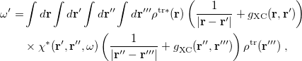
In vertical excitation or ionization, the solute undergoes a sudden change in its charge distribution. Various microscopic motions of the solvent have characteristic times to reach certain polarization response, and fast part of the solvent response (electrons) can follow such a dynamic process while the remaining degrees of freedom (nuclei) remain unchanged as in the initial state. Such splitting of the solvent response gives rise to non-equilibrium solvation. In the literature, two different approaches have been developed for describing non-equilibrium solvent effects: the linear response (LR) approach [621, 622] and the state-specific (SS) approach [618, 623, 624, 625]. Both are implemented in Q-Chem [626], at the SCF level for vertical ionization and at the corresponding (CIS or TDDFT) level for vertical excitation. A brief introduction to these methods is given below, and users who utilize the non-equilibrium PCM features are asked to cite Refs. You:2015 and Mewes:2015.

The LR approach considers the solvation effects as a coupling between a pair of transitions, one for solute and the other for solvent. The transition frequencies when the interaction between the solute and solvent is turned on may be determined by considering such an interaction as a perturbation. In the framework of TDDFT, the solvent/solute interaction is given by [628]

$\begin{equation} \label{eq:LR-term} \begin{split} \omega ’ = & \int d\ensuremath{\mathbf{r}} \int d\ensuremath{\mathbf{r}}’ \int d\ensuremath{\mathbf{r}}” \int d\ensuremath{\mathbf{r}}”’ \rho ^{{\ensuremath{\mathrm{tr}}}*}(\ensuremath{\mathbf{r}}) \left(\frac{1}{|\ensuremath{\mathbf{r}}-\ensuremath{\mathbf{r}}'|} + g_{\ensuremath{\mathrm{XC}}}(\ensuremath{\mathbf{r}},\ensuremath{\mathbf{r}}’)\right) \\ & \times \chi ^{*}(\ensuremath{\mathbf{r}}’,\ensuremath{\mathbf{r}}”,\omega ) \left(\frac{1}{|\ensuremath{\mathbf{r}}''-\ensuremath{\mathbf{r}}'''|} + g^{}_{\ensuremath{\mathrm{XC}}}(\ensuremath{\mathbf{r}}”,\ensuremath{\mathbf{r}}”’)\right) \rho ^{\ensuremath{\mathrm{tr}}}(\ensuremath{\mathbf{r}}”’) \; , \end{split} \end{equation}$

(11.4)

where $\chi$ is the charge density response function of the solvent and $\rho ^{\ensuremath{\mathrm{tr}}}(\ensuremath{\mathbf{r}})$ is the solute’s transition density. This term accounts for a dynamical correction to the transition energy so that it is related to the response of the solvent to the charge density of the solute oscillating at the solute transition frequency ( $\omega$ ). Within a PCM, only classical Coulomb interactions are taken into account, and Eq. eq:LR-term becomes

$\begin{equation} \begin{split} \omega ’_{\ensuremath{\mathrm{PCM}}} = & \int d\ensuremath{\mathbf{r}} \int d\ensuremath{\mathbf{s}} \frac{\rho ^{{\ensuremath{\mathrm{tr}}}*}(\ensuremath{\mathbf{r}})}{|\ensuremath{\mathbf{r}}-\ensuremath{\mathbf{s}}|} \int d\ensuremath{\mathbf{s}}’ \int d\ensuremath{\mathbf{r}}’ \, \mathcal{Q}(\ensuremath{\mathbf{s}},\ensuremath{\mathbf{s}}’,\varepsilon ) \frac{\rho ^{\ensuremath{\mathrm{tr}}}(\ensuremath{\mathbf{r}}')}{|\ensuremath{\mathbf{s}}'-\ensuremath{\mathbf{r}}'|} \; , \end{split} \end{equation}$

(11.7)

where $\mathcal{Q}$ is PCM solvent response operator for a generic dielectric constant, $\varepsilon$ . The integral of $\mathcal{Q}$ and the potential of the density $\rho ^{\ensuremath{\mathrm{tr}}}$ gives the surface charge density for the solvent polarization.

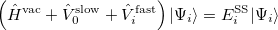
The state-specific (SS) approach takes into account the capability of a part of the solvent degrees of freedom to respond instantaneously to changes in the solute wave function upon excitation. Such an effect is not accounted for in the LR approach. In SS, a generic solvated-solute excited state $\Psi _ i$ is obtained as a solution of a nonlinear Schrödinger equation

$\begin{equation} \label{eq:SS-sdeq} \left(\hat{H}^{\ensuremath{\mathrm{vac}}} + \hat{V}^{\ensuremath{\mathrm{slow}}}_0 + \hat{V}^{\ensuremath{\mathrm{fast}}}_ i\right) |\Psi _ i\ensuremath{\rangle }= E^{\ensuremath{\mathrm{SS}}}_ i |\Psi _ i\ensuremath{\rangle }\end{equation}$

(11.9)

that depends upon the solute’s charge distribution. Here $\hat{H}^{\ensuremath{\mathrm{vac}}}$ is the usual Hamiltonian for the solute in vacuum and the reaction field operator $\hat{V}_ i$ generates the electrostatic potential of the apparent surface charge density (Section 11.2.2.1), corresponding to slow and fast polarization response. The solute is polarized self-consistently with respect to the solvent’s reaction field. In case of vertical ionization rather than excitation, both the ionized and non-ionized states can be treated within a ground-state formalism. For vertical excitations, self-consistent SS models [625, 629] have been developed for various excited-state methods, including both CIS and TDDFT.

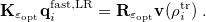
In a linear dielectric medium, the solvent polarization is governed by the electric susceptibility, $\chi = [\varepsilon (\omega ) - 1]/4\pi$ , where $\varepsilon (\omega )$ is the frequency-dependent permittivity, In case of very fast vertical transitions, the dielectric response is ruled by the optical dielectric constant, $\varepsilon _{\ensuremath{\mathrm{opt}}} = n^2$ , where $n$ is the solvent’s index of refraction. In both LR and SS, the fast part of the solvent’s degrees of freedom is in equilibrium with the solute density change. Within PCM, the fast solvent polarization charges for the SS excited state $i$ can be obtained by solving the following equation [624]:

$\begin{equation} \label{eq:Kq=Rv-fast} \ensuremath{\mathbf{K}}_{\varepsilon _{\ensuremath{\mathrm{opt}}}} \ensuremath{\mathbf{q}}^{\ensuremath{\mathrm{fast,SS}}}_ i = \ensuremath{\mathbf{R}}_{\varepsilon _{\ensuremath{\mathrm{opt}}}}\left[\ensuremath{\mathbf{v}}_ i + \ensuremath{\mathbf{v}}(\ensuremath{\mathbf{q}}^{\ensuremath{\mathrm{slow}}}_0)\right] \; . \end{equation}$

(11.10)

Here $\ensuremath{\mathbf{q}}^{\ensuremath{\mathrm{fast,SS}}}$ is the discretized fast surface charge. The dielectric constants in the matrices $\ensuremath{\mathbf{K}}$ and $\ensuremath{\mathbf{R}}$ (Section 11.2.2.1) are replaced with the optical dielectric constant, and $\ensuremath{\mathbf{v}}_ i$ is the potential of the solute’s excited state density, $\rho _ i$ . 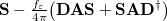The quantity $\ensuremath{\mathbf{v}}(\ensuremath{\mathbf{q}}^{\ensuremath{\mathrm{slow}}}_0)$ is the potential of the slow part of the apparent surface charges in the ground state, which are given by

$\begin{equation} \ensuremath{\mathbf{q}}^{\ensuremath{\mathrm{slow}}}_0 = \frac{\varepsilon - \varepsilon _{\ensuremath{\mathrm{opt}}}}{\varepsilon - 1}\ensuremath{\mathbf{q}}_0 \; . \end{equation}$

(11.11)

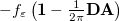
For LR-PCM, the solvent polarization is subjected to the first-order changes to the electron density (TDDFT linear density response), and thus Eq. eq:Kq=Rv-fast becomes

$\begin{equation} \ensuremath{\mathbf{K}}_{\varepsilon _{\ensuremath{\mathrm{opt}}}} \ensuremath{\mathbf{q}}^{\ensuremath{\mathrm{fast,LR}}}_ i = \ensuremath{\mathbf{R}}_{\varepsilon _{\ensuremath{\mathrm{opt}}}}\ensuremath{\mathbf{v}}(\rho ^{\ensuremath{\mathrm{tr}}}_ i) \; . \end{equation}$

(11.12)

The LR approach for CIS/TDDFT excitations and the self-consistent SS method (using the ground-state SCF) for vertical ionizations are available in Q-Chem. The self-consistent SS method for vertical excitations is not available, because this method is problematic in the vicinity of (near-) degeneracies between excited states, such as in the vicinity of a conical intersection. The fundamental problem in the SS approach is that each wave functional $\Psi _ i$ is an eigenfunction of a different Hamiltonian, since Eq. eq:SS-sdeq depend upon the specific state of interest. To avoid the ordering and the non-orthogonality problems, we compute the vertical excitation energy using a first-order, perturbative approximation to the SS approach [630, 631], in what we have termed the "ptSS" method [627]. The zeroth-order excited-state wavefunction can be calculated using various excited-state methods (currently available for CIS and TDDFT in Q-Chem) with solvent-relaxed molecular orbitals obtained from a ground-state PCM calculation. As mentioned previously, LR and SS describe different solvent relaxation features in non-equilibrium solvation. In the perturbation scheme, we can calculate the LR contribution using the zeroth-order transition density, in what we have called the "ptLR" approach. The combination of ptSS and ptLR yields quantitatively good solvatochromatic shifts, as compared to experimental results [626, 627].

The LR and SS approaches can also be used in the study of photon emission processes [632]. An emission process can be treated as a vertical excitation at a stationary point on the excited-state potential surface. The basic requirement therefore is to prepare the solvent-relaxed geometry for the excited-state of interest. TDDFT/C-PCM analytic gradients and Hessian are available in Q-Chem; see Section 6.3.5 for computational details regarding excited-state geometry optimization with PCM. An emission process is slightly more complicated than the absorption case. Two scenarios are discussed in literature, depending on the lifetime of an excited state in question. In the limiting case of ultrafast excited state decay, when only fast solvent degrees of freedom are expected to be equilibrated with the excited-state density. In this limit, the emission energy can be computed exactly in the same way as the vertical excitation energy. In this case, excited state geometry optimization should be performed in the non-equilibrium limit. The other limit is that of long-lived excited state, e.g., strongly fluorescent species and phosphorescence. In the long-lived case, excited state geometry optimization should be performed with the solvent equilibrium limit. Thus, the excited state should be computed using an equilibrium LR or SS apporach, and the ground state is calculated using non-equilibrium self-consistent SS approach.

11.2.3 PCM Job Control

A PCM calculation is requested by setting SOLVENT_METHOD = PCM in the $rem section. As mentioned above, there are a variety of different theoretical models that fall within the PCM family, so additional fine-tuning may be required, as described below.

11.2.3.1 $pcm section

Most PCM job control is accomplished via options specified in the $pcm input section, which allows the user to specify which flavor of PCM will be used, which algorithm will be used to solve the PCM equations, and other options. The format of the $pcm section is analogous to that of the $rem section:

$pcm
   <Keyword>  <parameter/option>
$end

NOTE: The following job control variables belong only in the $pcm section. Do not place them in the $rem section.

Theory

Specifies the which polarizable continuum model will be used.

INPUT SECTION: $pcm
TYPE:

STRING

DEFAULT:

CPCM

OPTIONS:

CPCM

Conductor-like PCM with $f_\varepsilon = (\varepsilon -1)/\varepsilon$ .

COSMO

Original conductor-like screening model with $f_\varepsilon = (\varepsilon -1)/(\varepsilon +1/2)$ .

IEFPCM

IEF-PCM with an asymmetric $\mathbf{K}$ matrix.

SSVPE

SS(V)PE model, equivalent to IEF-PCM with a symmetric $\mathbf{K}$ matrix.

RECOMMENDATION:

The IEF-PCM/SS(V)PE model is more sophisticated model than either C-PCM or COSMO, and probably more appropriate for low-dielectric solvents, but it is also more computationally demanding. In high-dielectric solvents there is little difference between these models. Note that the keyword COSMO in this context simply affects the dielectric screening factor $f_\varepsilon$ ; to obtain the outlying charge correction suggested by Klamt [599, 600], one should use SOLVENT_METHOD = COSMO rather than SOLVENT_METHOD = PCM. (See Section 11.2.6.)

Method

Specifies which surface discretization method will be used.

INPUT SECTION: $pcm
TYPE:

STRING

DEFAULT:

SWIG

OPTIONS:

SWIG

Switching/Gaussian method

ISWIG

“Improved” Switching/Gaussian method with an alternative switching function

Spherical

Use a single, fixed sphere for the cavity surface.

Fixed

Use discretization point charges instead of smooth Gaussians.

RECOMMENDATION:

Use of SWIG is recommended only because it is slightly more efficient than the switching function of ISWIG. On the other hand, ISWIG offers some conceptually more appealing features and may be superior in certain cases. Consult Refs. Lange:2010b,Lange:2011a for a discussion of these differences. The Fixed option uses the Variable Tesserae Number (VTN) algorithm of Li and Jensen [633], with Lebedev grid points. VTN uses point charges with no switching function or Gaussian blurring, and is therefore subject to discontinuities in geometry optimizations. It is not recommended, except to make contact with other calculations in the literature.

SwitchThresh

The threshold for discarding grid points on the cavity surface.

INPUT SECTION: $pcm
TYPE:

INTEGER

DEFAULT:

8

OPTIONS:

$n$

Discard grid points when the switching function is less than $10^{-n}$ .

RECOMMENDATION:

Use the default, which is found to avoid discontinuities within machine precision. Increasing $n$ reduces the cost of PCM calculations but can introduce discontinuities in the potential energy surface.

Construction of the solute cavity is an important part of the model and users should consult the literature in this capacity, especially with regard to the radii used for the atomic spheres. The default values provided in Q-Chem correspond to the consensus choice that has emerged over several decades, namely, to use van der Waals radii scaled by a factor of 1.2. The most widely-used set of van der Waals radii are those determined from crystallographic data by Bondi [619], although the radius for hydrogen was later adjusted to 1.1 [634]. Bondi’s analysis was later extended to the whole main group [635], and this entire extended set of van der Waals radii is available in Q-Chem. (For simplicity, we call these “Bondi radii” regardless of whether they come from Bondi’s original paper or the later work.) Alternatively, atomic radii from the Universal Force Field (UFF) are available [636]. The main appeal of UFF radii is that they are defined for all atoms of the periodic table, though the quality of these radii for PCM applications is unclear. Finally, the user may specify his or her own radii for cavity construction using a $van_der_waals input section, the format for which is described in Section 11.2.8. No scaling factor is applied to user-defined radii. Note that $R=0$ is allowed for a particular atomic radius, in which case the atom in question is not used to construct the cavity surface. This feature facilitates the construction of “united atom” cavities, in which the hydrogen atoms do not get their own spheres and the heavy-atom radii are increased to compensate [603].

Scaling the atomic radii is a crude way to account for the fact that solvent molecules should not typically penetrate all the way to the van der Waals radii of the solute. Another way to account for this effect is to employ a “solvent-accessible” cavity surface, which is constructed from the van der Waals surface by adding a certain value to each atomic radius. This value is the presumed radius of a solvent molecule. (The value 1.4 is often used for water.) The capability to specify a solvent “probe” radius to be added to the atomic radii of choice is available in Q-Chem.

Radii

Specifies which set of atomic van der Waals radii will be used to define the solute cavity.

INPUT SECTION: $pcm
TYPE:

STRING

DEFAULT:

BONDI

OPTIONS:

BONDI

Use the (extended) set of Bondi radii.

FF

Use Lennard-Jones radii from a molecular mechanics force field.

UFF

Use radii form the Universal Force Field.

READ

Read the atomic radii from a $van_der_waals input section.

RECOMMENDATION:

Bondi radii are widely used. The FF option requires the user to specify an MM force field using the FORCE_FIELD $rem variable, and also to define the atom types in the $molecule section (see Section 11.3). This is not required for UFF radii.

vdwScale

Scaling factor for the atomic van der Waals radii used to define the solute cavity.

INPUT SECTION: $pcm
TYPE:

FLOAT

DEFAULT:

1.2

OPTIONS:

$f$

Use a scaling factor of $f > 0$ .

RECOMMENDATION:

The default value is widely used in PCM calculations, although a value of 1.0 might be appropriate if using a solvent-accessible surface.

SASrad

Form a “solvent accessible” surface with the given solvent probe radius.

INPUT SECTION: $pcm
TYPE:

FLOAT

DEFAULT:

None

OPTIONS:

$r$

Use a solvent probe radius of $r$ , in .

RECOMMENDATION:

The solvent probe radius is added to the scaled van der Waals radii of the solute atoms. A common solvent probe radius for water is 1.4 , but the user should consult the literature regarding the use of solvent-accessible surfaces.

Historically, discretization of the cavity surface has involved “tessellation” methods that divide the cavity surface area into finite polygonal “tesserae”. (The GEPOL algorithm [637] is perhaps the most widely-used tessellation scheme.) Tessellation methods, however, suffer not only from discontinuities in the cavity surface area and solvation energy as a function of the nuclear coordinates, but in addition they lead to analytic energy gradients that are complicated to derive and implement. To avoid these problems, Q-Chem’s SWIG PCM implementation [591, 592, 593] uses Lebedev grids to discretize the atomic spheres. These are atom-centered grids with icosahedral symmetry, and may consist of anywhere from 26 to 5294 grid points per atomic sphere. The default values used by Q-Chem were selected based on extensive numerical tests [592, 593]. The default for MM atoms (in MM/PCM or QM/MM/PCM jobs) is $N=110$ Lebedev points per atomic sphere, whereas the default for QM atoms is $N=302$ . (This represents a change relative to Q-Chem versions earlier than 4.2.1, where the default for QM atoms was $N=590$ .) These default values exhibit good rotational invariance and absolute solvation energies that, in most cases, lie within $\sim$ 0.5–1.0 kcal/mol of the $N\rightarrow \infty$ limit [592], although exceptions (especially where charged solutes are involved) can be found [593]. The acceptable values for the number of Lebedev points per sphere are $N=26$ , 50, 110, 194, 302, 434, 590, 770, 974, 1202, 1454, 1730, 2030, 2354, 2702, 3074, 3470, 3890, 4334, 4802, or 5294.

HPoints

The number of Lebedev grid points to be placed on H atoms in the QM system.

INPUT SECTION: $pcm
TYPE:

INTEGER

DEFAULT:

302

OPTIONS:

Acceptable values are listed above.

RECOMMENDATION:

Use the default for geometry optimizations. For absolute solvation energies, the user may want to examine convergence with respect to $N$ .

HeavyPoints

The number of Lebedev grid points to be placed non-hydrogen atoms in the QM system.

INPUT SECTION: $pcm
TYPE:

INTEGER

DEFAULT:

302

OPTIONS:

Acceptable values are listed above.

RECOMMENDATION:

Use the default for geometry optimizations. For absolute solvation energies, the user may want to examine convergence with respect to $N$ .

MMHPoints

The number of Lebedev grid points to be placed on H atoms in the MM subsystem.

INPUT SECTION: $pcm
TYPE:

INTEGER

DEFAULT:

110

OPTIONS:

Acceptable values are listed above.

RECOMMENDATION:

Use the default for geometry optimizations. For absolute solvation energies, the user may want to examine convergence with respect to $N$ . This option applies only to MM/PCM or QM/MM/PCM calculations.

MMHeavyPoints

The number of Lebedev grid points to be placed on non-hydrogen atoms in the MM subsystem.

INPUT SECTION: $pcm
TYPE:

INTEGER

DEFAULT:

110

OPTIONS:

Acceptable values are listed above.

RECOMMENDATION:

Use the default for geometry optimizations. For absolute solvation energies, the user may want to examine convergence with respect to $N$ . This option applies only to MM/PCM or QM/MM/PCM calculations.

Especially for complicated molecules, the user may want to visualize the cavity surface. This can be accomplished by setting PrintLevel $\ge 2$ , which will trigger the generation of several “.PQR” files that describe the cavity surface. (These are written to the Q-Chem output file.) The .PQR format is similar to the common .PDB (Protein Data Bank) format, but also contains charge and radius information for each atom. One of the output .PQR files contains the charges computed in the PCM calculation and radii (in ) that are half of the square root of the surface area represented by each surface grid point. Thus, in examining this representation of the surface, larger discretization points are associated with larger surface areas. A second .PQR file contains the solute’s electrostatic potential (in atomic units), in place of the charge information, and uses uniform radii for the grid points. These .PQR files can be visualized using various third-party software, including the freely-available Visual Molecular Dynamics (VMD) program [487, 488], which is particularly useful for coloring the .PQR surface grid points according to their charge, and sizing them according to their contribution to the molecular surface area. (Examples of such visualizations can be found in Ref. Lange:2010a.)

PrintLevel

Controls the printing level during PCM calculations.

INPUT SECTION: $pcm
TYPE:

INTEGER

DEFAULT:

0

OPTIONS:

0

Prints PCM energy and basic surface grid information. Minimal additional printing.

1

Level 0 plus PCM solute-solvent interaction energy components and Gauss’ Law error.

2

Level 1 plus surface grid switching parameters and a .PQR file for visualization of

the cavity surface apparent surface charges.

3

Level 2 plus a .PQR file for visualization of the electrostatic potential at the surface

grid created by the converged solute.

4

Level 3 plus additional surface grid information, electrostatic potential and apparent

surface charges on each SCF cycle.

5

Level 4 plus extensive debugging information.

RECOMMENDATION:

Use the default unless further information is desired.

Finally, note that setting Method to Spherical in the $pcm input selection requests the construction of a solute cavity consisting of a single, fixed sphere. This is generally not recommended but is occasionally useful for making contact with the results of Born models in the literature, or the Kirkwood-Onsager model discussed in Section 11.2.1. In this case, the cavity radius and its center must also be specified in the $pcm section. The keyword HeavyPoints controls the number of Lebedev grid points used to discretize the surface.

CavityRadius

Specifies the solute cavity radius.

INPUT SECTION: $pcm
TYPE:

FLOAT

DEFAULT:

None

OPTIONS:

$R$

Use a radius of $R$ , in Angstroms.

RECOMMENDATION:

None.

CavityCenter

Specifies the center of the spherical solute cavity.

INPUT SECTION: $pcm
TYPE:

FLOAT

DEFAULT:

0.0 0.0 0.0

OPTIONS:

$x$ $y$ $z$

Coordinates of the cavity center, in Angstroms.

RECOMMENDATION:

The format is CavityCenter followed by three floating-point values, delineated by spaces. Uses the same coordinate system as the $molecule section.

11.2.3.2 Examples

The following example shows a very basic PCM job. The solvent dielectric is specified in the $solvent section, which is described below.

Example 11.242 A basic example of using the PCMs: optimization of trifluoroethanol in water.

$rem
JOBTYPE         OPT
BASIS           6-31G*
METHOD          B3LYP
SOLVENT_METHOD  PCM
$end

$pcm
Theory          CPCM
Method          SWIG
Solver          Inversion
HeavyPoints     194
HPoints         194
Radii           Bondi
vdwScale        1.2
$end

$solvent
Dielectric 78.39
$end

$molecule
0 1
  C    -0.245826    -0.351674    -0.019873
  C     0.244003     0.376569     1.241371
  O     0.862012    -0.527016     2.143243
  F     0.776783    -0.909300    -0.666009
  F    -0.858739     0.511576    -0.827287
  F    -1.108290    -1.303001     0.339419
  H    -0.587975     0.878499     1.736246
  H     0.963047     1.147195     0.961639
  H     0.191283    -1.098089     2.489052
$end

The next example uses a single spherical cavity and should be compared to the Kirkwood-Onsager job, Example 11.11.1 on page *.

Example 11.243 PCM with a single spherical cavity, applied to H $_2$ O in acetonitrile

$molecule
0 1
O       0.00000000     0.00000000     0.11722303
H      -0.75908339     0.00000000    -0.46889211
H       0.75908339     0.00000000    -0.46889211
$end

$rem
method            HF
basis             6-31g**
solvent_method    pcm
$end

$pcm
method        spherical   ! single spherical cavity with 590 discretization points
HeavyPoints   590
CavityRadius  1.8         ! Solute Radius, in Angstrom
CavityCenter  0.0 0.0 0.0 ! Will be at center of Standard Nuclear Orientation
Theory        SSVPE
$end

$solvent
Dielectric        35.9   !   Acetonitrile
$end

Finally, we consider an example of a united-atom cavity. Note that a user-defined van der Waals radius is supplied only for carbon, so the hydrogen radius is taken to be zero and thus the hydrogen atoms are not used to construct the cavity surface. (As mentioned above, the format for the $van_der_waals input section is discussion in Section 11.2.8).

Example 11.244 United-atom cavity construction for ethylene.

$comment
Benzene (in benzene), with a united-atom cavity construction
R = 2.28 A for carbon, R = 0 for hydrogen
$end

$molecule
0 1
          C       1.3862000000     0.0000000000     0.0000000000
          C       0.6931000000     1.2004844147     0.0000000000
          C      -0.6931000000     1.2004844147     0.0000000000
          C      -1.3862000000     0.0000000000     0.0000000000
          C      -0.6931000000    -1.2004844147     0.0000000000
          C       0.6931000000    -1.2004844147     0.0000000000
          H       2.4618000000     0.0000000000     0.0000000000
          H       1.2309000000     2.1319813390     0.0000000000
          H      -1.2309000000     2.1319813390     0.0000000000
          H      -2.4618000000     0.0000000000     0.0000000000
          H      -1.2309000000    -2.1319813390     0.0000000000
          H       1.2309000000    -2.1319813390     0.0000000000
$end

$rem
exchange        hf
basis           6-31G*
solvent_method  pcm
$end

$pcm
theory          iefpcm   ! this is a synonym for ssvpe
method          swig
printlevel      1
radii           read
$end

$solvent
dielectric 2.27
$end

$van_der_waals
1
  6     2.28
$end

11.2.3.3 $solvent section

The solvent for PCM calculations is specified using the $solvent section, as documented below. In addition, the $solvent section can be used to incorporate non-electrostatic interaction terms into the solvation energy. (The Theory keyword in the $pcm section specifies only how the electrostatic interactions are handled.) The general form of the $solvent input section is shown below. The $solvent section was used above to specify parameters for the Kirkwood-Onsager SCRF model, and will be used again below to specify the solvent for SM $x$ calculations (Section 11.2.7); in each case, the particular options that can be listed in the $solvent section depend upon the value of the $rem variable SOLVENT_METHOD.

$solvent
   NonEls  <Option>
   NSolventAtoms <Number unique of solvent atoms>
   SolventAtom <Number1> <Number2> <Number3> <SASrad>
   SolventAtom <Number1> <Number2> <Number3> <SASrad>
   . . .
   <Keyword>  <parameter/option>
   . . .
$end

The keyword SolventAtom requires multiple parameters, whereas all other keywords require only a single parameter. In addition to any (optional) non-electrostatic parameters, the $solvent section is also used to specify the solvent’s dielectric constant. If non-electrostatic interactions are ignored, then this is the only keyword that is necessary in the $solvent section. For non-equilibrium TD-DFT/C-PCM calculations (Section 11.2.2.3), the optical dielectric constant should be specified in the $solvent section as well.

Dielectric

The (static) dielectric constant of the PCM solvent.

INPUT SECTION: $solvent
TYPE:

FLOAT

DEFAULT:

78.39

OPTIONS:

$\varepsilon$

Use a dielectric constant of $\varepsilon > 0$ .

RECOMMENDATION:

The static (i.e., zero-frequency) dielectric constant is what is usually called “the” dielectric constant. The default corresponds to water at 25 $^\circ$ C.

OpticalDielectric

The optical dielectric constant of the PCM solvent.

INPUT SECTION: $solvent
TYPE:

FLOAT

DEFAULT:

1.78

OPTIONS:

$\varepsilon _\infty$

Use an optical dielectric constant of $\varepsilon _\infty > 0$ .

RECOMMENDATION:

The default corresponds to water at 25 $^\circ$ C. Note that $\varepsilon _\infty = n^2$ , where $n$ is the solvent’s index of refraction.

The non-electrostatic interactions currently available in Q-Chem are based on the work of Cossi et al. [638], and are computed outside of the SCF procedure used to determine the electrostatic interactions. The non-electrostatic energy is highly dependent on the input parameters and can be extremely sensitive to the radii chosen to define the solute cavity. Accordingly, the inclusion of non-electrostatic interactions is highly empirical and probably needs to be considered on a case-by-case basis. Following Ref. Cossi:1996, the cavitation energy is computed using the same solute cavity that is used to compute the electrostatic energy, whereas the dispersion/repulsion energy is computed using a solvent-accessible surface.

The following keywords (in the $solvent section) are used to define non-electrostatic parameters for PCM calculations.

NonEls

Specifies what type of non-electrostatic contributions to include.

INPUT SECTION: $solvent
TYPE:

STRING

DEFAULT:

None

OPTIONS:

Cav

Cavitation energy

Buck

Buckingham dispersion and repulsion energy from atomic number

LJ

Lennard-Jones dispersion and repulsion energy from force field

BuckCav

Buck + Cav

LJCav

LJ + Cav

RECOMMENDATION:

A very limited set of parameters for the Buckingham potential is available at present.

NSolventAtoms

The number of different types of atoms.

INPUT SECTION: $solvent
TYPE:

INTEGER

DEFAULT:

None

OPTIONS:

$N$

Specifies that there are $N$ different types of atoms.

RECOMMENDATION:

This keyword is necessary when NonEls = Buck, LJ, BuckCav, or LJCav. Methanol ( $\rm CH_3OH$ ), for example, has three types of atoms (C, H, and O).

SolventAtom

Specifies a unique solvent atom.

INPUT SECTION: $solvent
TYPE:

Various

DEFAULT:

None.

OPTIONS:

Input (TYPE)

Description

Number1 (INTEGER):

The atomic number of the atom

Number2 (INTEGER):

How many of this atom are in a solvent molecule

Number3 (INTEGER):

Force field atom type

SASrad (FLOAT):

Probe radius (in ) for defining the solvent accessible surface

RECOMMENDATION:

If not using LJ or LJCav, Number3 should be set to 0. The SolventAtom keyword is necessary when NonEls = Buck, LJ, BuckCav, or LJCav.

Temperature

Specifies the solvent temperature.

INPUT SECTION: $solvent
TYPE:

FLOAT

DEFAULT:

300.0

OPTIONS:

$T$

Use a temperature of $T$ , in Kelvin.

RECOMMENDATION:

Used only for the cavitation energy.

Pressure

Specifies the solvent pressure.

INPUT SECTION: $solvent
TYPE:

FLOAT

DEFAULT:

1.0

OPTIONS:

$P$

Use a pressure of $P$ , in bar.

RECOMMENDATION:

Used only for the cavitation energy.

SolventRho

Specifies the solvent number density

INPUT SECTION: $solvent
TYPE:

FLOAT

DEFAULT:

Determined for water, based on temperature.

OPTIONS:

$\rho$

Use a density of $\rho$ , in molecules/ $^3$ .

RECOMMENDATION:

Used only for the cavitation energy.

SolventRadius

The radius of a solvent molecule of the PCM solvent.

INPUT SECTION: $solvent
TYPE:

FLOAT

DEFAULT:

None

OPTIONS:

$r$

Use a radius of $r$ , in .

RECOMMENDATION:

Used only for the cavitation energy.

The following example illustrates the use of the non-electrostatic interactions.

Example 11.245 Optimization of trifluoroethanol in water using both electrostatic and non-electrostatic PCM interactions. OPLSAA parameters are used in the Lennard-Jones potential for dispersion and repulsion.

$rem
JOBTYPE        OPT
BASIS          6-31G*
METHOD         B3LYP
SOLVENT_METHOD PCM
FORCE_FIELD    OPLSAA
$end

$pcm
Theory      CPCM
Method      SWIG
Solver      Inversion
HeavyPoints 194
HPoints     194
Radii       Bondi
vdwScale    1.2
$end

$solvent
NonEls        LJCav
NSolventAtoms 2
SolventAtom   8 1 186 1.30
SolventAtom   1 2 187 0.01
SolventRadius 1.35
Temperature   298.15
Pressure      1.0
SolventRho    0.03333
Dielectric    78.39
$end

$molecule
0 1
  C    -0.245826    -0.351674    -0.019873     23
  C     0.244003     0.376569     1.241371     22
  O     0.862012    -0.527016     2.143243     24
  F     0.776783    -0.909300    -0.666009     26
  F    -0.858739     0.511576    -0.827287     26
  F    -1.108290    -1.303001     0.339419     26
  H    -0.587975     0.878499     1.736246     27
  H     0.963047     1.147195     0.961639     27
  H     0.191283    -1.098089     2.489052     25
$end

11.2.3.4 Job control and Examples for Non-Equilibrium Solvation

The OpticalDielectric keyword in $solvent is always needed. The LR energy is automatically calculated while the CIS/TDDFT calculations are performed with PCM, but it is turned off while the perturbation scheme is employed.

ChargeSeparation

Partition fast and slow charges in solvent equilibrium state

INPUT SECTION: $pcm
TYPE:

STRING

DEFAULT:

No default.

OPTIONS:

Marcus

Do slow-fast charge separation in the ground state.

Excited

Do slow-fast charge separation in an excited-state.

RECOMMENDATION:

Charge separation is used in conjunction with the StateSpecific keyword in $pcm.

StateSpecific

Specifies which the state-specific method will be used.

INPUT SECTION: $pcm
TYPE:

Various

DEFAULT:

No default.

OPTIONS:

Ground

Run self-consistent SS method in the ground-state with a given slow polarization charges.

Perturb

Perform ptSS and ptLR for vertical excitations.

$i$

The $i$ -th excited-state used for charge separation (for emission).

RECOMMENDATION:

NoneqGrad

Control whether perform excited state geometry optimization in equilibrium or non-equilibrium.

INPUT SECTION: $pcm
TYPE:

NONE

DEFAULT:

No default.

OPTIONS:

RECOMMENDATION:

Specify it for non-equilibrium optimization otherwise equilibrium geometry optimization will be performed.

Example 11.246 LR-TDDFT/C-PCM low-lying vertical excitation energy

$molecule
 0 1
  C           0  0  0.0
  O           0  0  1.21
$end

$rem
  EXCHANGE            B3LP
  CIS_N_ROOTS         10
  CIS_SINGLETS        TRUE
  CIS_TRIPLETS	      TRUE
  RPA                 TRUE
  BASIS               6-31+G*
  SOLVENT_METHOD      PCM
$end

$pcm
  Theory      CPCM
  Method      SWIG
  Solver      Inversion
  Radii       Bondi
$end

$solvent
  Dielectric         78.39
  OpticalDielectric  1.777849
$end

Example 11.247 PCM solvation effects on the vertical excitation energies of planar DMABN using the ptSS and ptLR methods.

$molecule
 0  1
  C         0.0000466670   -0.0003989920    1.9049533013
  C         1.2100273911    0.0003798174    1.1860514263
  C         1.2146402411   -0.0000659664   -0.1945152488
  C         0.0001642918   -0.0006163800   -0.9338323670
  C        -1.2143493593   -0.0015573129   -0.1946877858
  C        -1.2097539311   -0.0018468783    1.1857751832
  H         2.1519498961    0.0013779318    1.7220180544
  H         2.1643711416    0.0004818107   -0.7096402413
  H        -2.1640827320   -0.0020086712   -0.7097815919
  H        -2.1517638721   -0.0022872146    1.7216153743
  C        -0.0002270265    0.0010614144    3.3253023786
  N        -0.0004752169    0.0024050570    4.4843211392
  N         0.0000539889   -0.0001561808   -2.2973728307
  C        -1.2586568849    0.0012846735   -3.0369947926
  H        -1.0410420397    0.0016150528   -4.1023766685
  H        -1.8608970185   -0.8856472814   -2.8111179665
  H        -1.8592477277    0.8891330458   -2.8102379603
  C         1.2585638668   -0.0006605040   -3.0372852058
  H         1.8606513946    0.8862082585   -2.8107557102
  H         1.8593622362   -0.8886046730   -2.8114618382
  H         1.0406646935   -0.0000970072   -4.1026090234
$end

$rem
  JOBTYPE               SP
  EXCHANGE              LRC-wPBEPBE
  OMEGA                 260
  BASIS                 6-31G*
  CIS_N_ROOTS           10
  RPA                   2
  CIS_SINGLETS          1
  CIS_TRIPLETS          0

  CIS_DYNAMIC_MEM       TRUE
  CIS_RELAXED_DENSITY   TRUE
  USE_NEW_FUNCTIONAL    TRUE

  SOLVENT_METHOD        PCM
  PCM_PRINT             1
$end

$pcm
 Theory                 IEFPCM
 ChargeSeparation       Marcus
 StateSpecific          Perturb
$end

$solvent
 Dielectric             35.688000       ! Acetonitrile
 OpticalDielectric      1.806874
$end

Example 11.248 Aqueous phenol ionization using state-specific non-equilibrium PCM

$molecule
 0  1
  C -0.189057 -1.215927 -0.000922
  H -0.709319 -2.157526 -0.001587
  C  1.194584 -1.155381 -0.000067
  H  1.762373 -2.070036 -0.000230
  C  1.848872  0.069673  0.000936
  H  2.923593  0.111621  0.001593
  C  1.103041  1.238842  0.001235
  H  1.595604  2.196052  0.002078
  C -0.283047  1.185547  0.000344
  H -0.862269  2.095160  0.000376
  C -0.929565 -0.042566 -0.000765
  O -2.287040 -0.159171 -0.001759
  H -2.663814  0.725029  0.001075
$end

$rem
  JOBTYPE               SP
  EXCHANGE              wPBE
  CORRELATION           PBE
  LRC_DFT               1
  OMEGA                 300
  BASIS                 6-31+G*
  SCF_CONVERGENCE       8
  SOLVENT_METHOD        PCM
  PCM_PRINT             1
$end

$pcm
  ChargeSeparation      Marcus
$end

$solvent
  Dielectric            78.39
  OpticalDielectric     1.777849
$end

@@@
$molecule
 1  2
 READ
$end

$rem
  JOBTYPE               SP
  EXCHANGE              wPBE
  CORRELATION           PBE
  LRC_DFT               1
  OMEGA                 300
  BASIS                 6-31+G*
  SCF_CONVERGENCE       8
  SOLVENT_METHOD        PCM
  PCM_PRINT             1
  SCF_GUESS             READ
$end

$pcm
  StateSpecific         Ground
$end

$solvent
  Dielectric            78.39
  OpticalDielectric     1.777849
$end

Example 11.249 PCM solvation effects on the emission energy of twisted DMABN in acetonitrile.

$molecule
 0  1
  C        -0.0000020664   -0.0000030657    1.8944472102
  C         1.2301788386    0.0000034932    1.1607654421
  C         1.2448623254    0.0000019224   -0.2003601210
  C         0.0000035154   -0.0000130458   -0.9179014646
  C        -1.2448450017   -0.0000007858   -0.2003542615
  C        -1.2301606293    0.0000009019    1.1607531534
  H         2.1711288221    0.0000135363    1.7040640230
  H         2.1806701315    0.0000099280   -0.7501405321
  H        -2.1806573730    0.0000061271   -0.7501203529
  H        -2.1711120141    0.0000069286    1.7040377372
  C        -0.0000236776   -0.0000026392    3.2935096257
  N        -0.0000117329   -0.0000010959    4.4594155390
  N        -0.0000087428   -0.0000059515   -2.3091936565
  C         0.0000010176    1.2538813765   -3.0212357565
  H         0.0000057176    1.0990763913   -4.0986604824
  H        -0.8829081343    1.8189750963   -2.7058150336
  H         0.8829113886    1.8189675327   -2.7058056136
  C        -0.0000093023   -1.2538863802   -3.0212468120
  H         0.8829172783   -1.8189662532   -2.7058494734
  H        -0.8829018393   -1.8189927074   -2.7058033199
  H        -0.0000385216   -1.0990713095   -4.0986701147
$end

$rem
  JOBTYPE               SP
  EXCHANGE              LRC-wPBEPBE
  OMEGA                 280
  BASIS                 6-31G*
  CIS_N_ROOTS           10
  RPA                   2
  CIS_SINGLETS          1
  CIS_TRIPLETS          0

  CIS_DYNAMIC_MEM       TRUE
  CIS_RELAXED_DENSITY   TRUE
  USE_NEW_FUNCTIONAL    TRUE

  SOLVENT_METHOD        PCM
  PCM_PRINT             1
$end

$pcm
 ChargeSeparation       Excited
 StateSpecific          1
$end

$solvent
 Dielectric             35.688000   ! Acetonitrile
 OpticalDielectric      1.806874
$end

@@@
$molecule
  READ
$end

$rem
  JOBTYPE               SP
  EXCHANGE              LRC-wPBEPBE
  OMEGA                 280
  BASIS                 6-31G*
  SCF_GUESS             READ
  SCF_CONVERGENCE       8

  SOLVENT_METHOD        PCM
  PCM_PRINT             1
$end

$pcm
 StateSpecific          Ground
$end

$solvent
 Dielectric             35.688000   ! Acetonitrile
 OpticalDielectric      1.806874
$end

11.2.4 Linear-Scaling QM/MM/PCM Calculations

Recall that PCM electrostatics calculations require the solution of the set of linear equations given in Eq. eq:Kq=Rv, to determine the vector $\mathbf{q}$ of apparent surface charges. The precise forms of the matrices $\mathbf{K}$ and $\mathbf{R}$ depend upon the particular PCM (Table 11.2), but in any case they have dimension $N_{grid}\times N_{grid}$ , where $N_{grid}$ is the number of Lebedev grid points used to discretize the cavity surface. Construction of the matrix $\mathbf{K}^{-1}\mathbf{R}$ affords a numerically exact solution to Eq. eq:Kq=Rv, whose cost scales as $\mbox{${\cal {O}}({N^3_{grid}})$}$ in CPU time and $\mbox{${\cal {O}}({N^2_{grid}})$}$ in memory. This cost is exacerbated by smooth PCMs, which discard fewer interior grid points so that $N_{grid}$ tends to be larger, for a given solute, as compared to traditional discretization schemes. For QM solutes, the cost of inverting $\mathbf{K}$ is usually negligible relative to the cost of the electronic structure calculation, but for the large values of $N_{grid}$ that are encountered in MM/PCM or QM/MM/PCM jobs, the $\mbox{${\cal {O}}({N^3_{grid}})$}$ cost of inverting $\mathbf{K}$ is often prohibitively expensive.

To avoid this bottleneck, Lange and Herbert [594] have developed an iterative conjugate gradient (CG) solver for Eq. eq:Kq=Rv whose cost scales as $\mbox{${\cal {O}}({N^2_{grid}})$}$ in CPU time and $\mbox{${\cal {O}}({N_{grid}})$}$ in memory. A number of other cost-saving options are available, including efficient pre-conditioners and matrix factorizations that speed up convergence of the CG iterations, and a fast multipole algorithm for computing the electrostatic interactions [639]. Together, these features lend themselves to a solution of Eq. eq:Kq=Rv whose cost scales as $\mbox{${\cal {O}}({N_{grid}^{}})$}$ in both memory and CPU time, for sufficiently large systems [594]. Currently, these options are available only for C-PCM, not for SS(V)PE/IEF-PCM.

Listed below are job control variables for the CG solver, which should be specified within the $pcm input section. Researchers who use this feature are asked to cite the original SWIG PCM references [592, 593] as well as the reference for the CG solver [594].

Solver

Specifies the algorithm used to solve the PCM equations.

INPUT SECTION: $pcm
TYPE:

STRING

DEFAULT:

INVERSION

OPTIONS:

INVERSION

Direct matrix inversion

CG

Iterative conjugate gradient

RECOMMENDATION:

Matrix inversion is faster for small solutes because it needs to be performed only once in a single-point calculation. However, the CG solver (which must be applied at each SCF iteration) is recommended for large MM/PCM or QM/MM/PCM calculations.

CGThresh

The threshold for convergence of the conjugate gradient solver.

INPUT SECTION: $pcm
TYPE:

INTEGER

DEFAULT:

6

OPTIONS:

$n$

Conjugate gradient converges when the maximum residual is less than $10^{-n}$ .

RECOMMENDATION:

The default typically affords PCM energies on par with the precision of matrix inversion for small systems. For systems that have difficulty with SCF convergence, one should increase $n$ or try the matrix inversion solver. For well-behaved or very large systems, a smaller $n$ might be permissible.

DComp

Controls decomposition of matrices to reduce the matrix norm for the CG Solver.

INPUT SECTION: $pcm
TYPE:

INTEGER

DEFAULT:

1

OPTIONS:

0

Turns off matrix decomposition

1

Turns on matrix decomposition

3

Option 1 plus only stores upper half of matrix and enhances gradient evaluation

RECOMMENDATION:

None

PreCond

Controls the use of the pre-conditioner for the CG solver.

INPUT SECTION: $pcm
TYPE:

None

DEFAULT:

Off

OPTIONS:

No options. Specify the keyword to enable pre-conditioning.

RECOMMENDATION:

A Jacobi block-diagonal pre-conditioner is applied during the conjugate gradient algorithm to improve the rate of convergence. This reduces the number of CG iterations, at the expense of some overhead. Pre-conditioning is generally recommended for large systems.

NoMatrix

Specifies whether PCM matrices should be explicitly constructed and stored.

INPUT SECTION: $pcm
TYPE:

None

DEFAULT:

Off

OPTIONS:

No options. Specify the keyword to avoid explicit construction of PCM matrices.

RECOMMENDATION:

Storing the PCM matrices requires $\mbox{${\cal {O}}({N_{grid}^2})$}$ memory. If this is prohibitive, the NoMatrix option forgoes explicit construction of the PCM matrices, and instead constructs the matrix elements as needed, reducing the memory requirement to $\mbox{${\cal {O}}({N_{grid}})$}$ at the expense of additional computation.

UseMultipole

Controls the use of the adaptive fast multipole method in the CG solver.

INPUT SECTION: $pcm
TYPE:

None

DEFAULT:

Off

OPTIONS:

No options. Specify the keyword in order to enable the fast multipole method.

RECOMMENDATION:

The fast multipole approach formally reduces the CPU time to $\mbox{${\cal {O}}({N_{grid}})$}$ , but is only beneficial for spatially extended systems with several thousand cavity grid points. Requires the use of NoMatrix.

MultipoleOrder

Specifies the highest multipole order to use in the FMM.

INPUT SECTION: $pcm
TYPE:

INTEGER

DEFAULT:

4

OPTIONS:

$n$

The highest order multipole in the multipole expansion.

RECOMMENDATION:

Increasing the multipole order improves accuracy but also adds more computational expense. The default yields satisfactory performance in common QM/MM/PCM applications.

Theta

The multipole acceptance criterion.

INPUT SECTION: $pcm
TYPE:

FLOAT

DEFAULT:

0.6

OPTIONS:

$n$

A number between zero and one.

RECOMMENDATION:

The default is recommended for general usage. This variable determines when the use of a multipole expansion is valid. For a given grid point and box center in the FMM, a multipole expansion is accepted when $r / d <=$ Theta, where $d$ is the distance from the grid point to the box center and $r$ is the radius of the box. Setting Theta to one will accept all multipole expansions, whereas setting it to zero will accept none. If not accepted, the grid point’s interaction with each point inside the box is computed explicitly. A low Theta is more accurate but also more expensive than a higher Theta.

NBox

The FMM boxing threshold.

INPUT SECTION: $pcm
TYPE:

INTEGER

DEFAULT:

100

OPTIONS:

$n$

The maximum number of grid points for a leaf box.

RECOMMENDATION:

The default is recommended. This option is for advanced users only. The adaptive FMM boxing algorithm divides space into smaller and smaller boxes until each box has less than or equal to NBox grid points. Modification of the threshold can lead to speedup or slowdown depending on the molecular system and other FMM variables.

A sample input file for the linear-scaling QM/MM/PCM methodology can be found in the $QC/samples directory, under the name QMMMPCM_crambin.in. This sample involves a QM/MM description of a protein (crambin) in which a single tyrosine side chain is taken to be the QM region. The entire protein is immersed in a dielectric using C-PCM with SWIG discretization.

11.2.5 Iso-Density Implementation of SS(V)PE

11.2.5.1 Basic job control

As discussed above, results obtained various types of PCMs are quite sensitive to the details of the cavity construction. Q-Chem’s implementation of PCMs, using Lebedev grids, simplifies this construction somewhat, but leaves the radii of the atomic spheres as empirical parameters (albeit ones for which widely-used default values are provided). An alternative implementation of the SS(V)PE solvation model is also available [602], which attempts to further eliminate empiricism associated with cavity construction by taking the cavity surface to be a specified iso-contour of the solute’s electron density. (We call this the isodensity implementation of SS(V)PE in Table 11.2, and it is based on Chipman’s “symmetrized” form of the $\mathbf{K}$ matrix [602, 593].) In this case, the cavity surface is discretized by projecting a single-center Lebedev grid onto the iso-contour surface. Unlike the PCM implementation discussed in Section 11.2.2, for which point-group symmetry is disabled, this implementation of SS(V)PE supports full symmetry for all Abelian point groups. The larger and/or the less spherical the solute molecule is, the more points are needed to get satisfactory precision in the results. Further experience will be required to develop detailed recommendations for this parameter. Values as small as 110 points are usually sufficient for diatomic or triatomic molecules. The default value of 1202 points is adequate to converge the energy within 0.1 kcal/mol for solutes the size of mono-substituted benzenes.

Although cavitation, dispersion, and and specific hydrogen-bonding corrections for use with the iso-density SS(V)PE model have been reported in the literature [604, 605], these are not yet available in Q-Chem. Energy gradients are also not available for this implementation of SS(V)PE, although they are available for the implementation described in Section 11.2.2 in which the cavity is constructed from atom-centered spheres. As with the PCMs discussed in that section, the solute may be described using Hartree-Fock theory or DFT; post-Hartree–Fock correlated wavefunctions can also take advantage of molecular orbitals that are polarized using SS(V)PE. Researchers who use the iso-density SS(V)PE feature are asked to cite Ref. Chipman:2000.

An iso-density SS(V)PE calculation is requested by setting SOLVENT_METHOD = ISOSVP in the $rem section, in addition to normal job control variables for a single-point energy calculation. Whereas the other solvation models described in this chapter use specialized input sections (e.g., $pcm) in lieu of a slew of $rem variables, the iso-density SS(V)PE code is an interface between Q-Chem and a stand-alone FORTRAN code written by Chipman [602], and some $rem variables are used for job control of isodensity SS(V)PE calculations. These are listed below.

SVP_MEMORY

Specifies the amount of memory for use by the solvation module.

TYPE:

INTEGER

DEFAULT:

125

OPTIONS:

$n$ corresponds to the amount of memory in MB.

RECOMMENDATION:

The default should be fine for medium size molecules with the default Lebedev grid, only increase if needed.

SVP_PATH

Specifies whether to run a gas phase computation prior to performing the solvation procedure.

TYPE:

INTEGER

DEFAULT:

0

OPTIONS:

0

runs a gas-phase calculation and after

convergence runs the SS(V)PE computation.

1

does not run a gas-phase calculation.

RECOMMENDATION:

Running the gas-phase calculation provides a good guess to start the solvation stage and provides a more complete set of solvated properties.

SVP_CHARGE_CONV

Determines the convergence value for the charges on the cavity. When the change in charges fall below this value, if the electron density is converged, then the calculation is considered converged.

TYPE:

INTEGER

DEFAULT:

7

OPTIONS:

$n$ Convergence threshold set to $10^{-n}$ .

RECOMMENDATION:

The default value unless convergence problems arise.

SVP_CAVITY_CONV

Determines the convergence value of the iterative iso-density cavity procedure.

TYPE:

INTEGER

DEFAULT:

10

OPTIONS:

$n$ Convergence threshold set to $10^{-n}$ .

RECOMMENDATION:

The default value unless convergence problems arise.

SVP_GUESS

Specifies how and if the solvation module will use a given guess for the charges and cavity points.

TYPE:

INTEGER

DEFAULT:

0

OPTIONS:

0

No guessing.

1

Read a guess from a previous Q-Chem solvation computation.

2

Use a guess specified by the $svpirf section from the input

RECOMMENDATION:

It is helpful to also set SCF_GUESS to READ when using a guess from a previous Q-Chem run.

This last $rem variable requires specification of a $svpirf input section, the format for which is the following:

$svpirf
   <# point> <x point>  <y point>  <z point>  <charge> <grid weight>
   <# point> <x normal> <y normal> <z normal>
$end

11.2.5.2 The $svp input section

More refined control over SS(V)PE jobs is obtained using a $svp input section. These are read directly by Chipman’s SS(V)PE solvation module and and therefore must be specified in the context of a FORTRAN namelist. The format is as follows:

$svp
   <KEYWORD>=<VALUE>, <KEYWORD>=<VALUE>,...
   <KEYWORD>=<VALUE>
$end

For example, the section may look like this:

$svp
   RHOISO=0.001, DIELST=78.39, NPTLEB=110
$end

The following keywords are supported in the $svp section:

DIELST

The static dielectric constant.

TYPE:

FLOAT

DEFAULT:

78.39

OPTIONS:

real number specifying the constant.

RECOMMENDATION:

The default value 78.39 is appropriate for water solvent.

ISHAPE

A flag to set the shape of the cavity surface.

TYPE:

INTEGER

DEFAULT:

0

OPTIONS:

0

use the electronic iso-density surface.

1

use a spherical cavity surface.

RECOMMENDATION:

Use the default surface.

RHOISO

Value of the electronic iso-density contour used to specify the cavity surface. (Only relevant for ISHAPE = 0).

TYPE:

FLOAT

DEFAULT:

0.001

OPTIONS:

Real number specifying the density in electrons/bohr $^3$ .

RECOMMENDATION:

The default value is optimal for most situations. Increasing the value produces a smaller cavity which ordinarily increases the magnitude of the solvation energy.

RADSPH

Sphere radius used to specify the cavity surface (Only relevant for ISHAPE=1).

TYPE:

FLOAT

DEFAULT:

Half the distance between the outermost atoms plus 1.4 Angstroms.

OPTIONS:

Real number specifying the radius in bohr (if positive) or in Angstroms (if negative).

RECOMMENDATION:

Make sure that the cavity radius is larger than the length of the molecule.

INTCAV

A flag to select the surface integration method.

TYPE:

INTEGER

DEFAULT:

0

OPTIONS:

0

Single center Lebedev integration.

1

Single center spherical polar integration.

RECOMMENDATION:

The Lebedev integration is by far the more efficient.

NPTLEB

The number of points used in the Lebedev grid for the single-center surface integration. (Only relevant if INTCAV=0).

TYPE:

INTEGER

DEFAULT:

1202

OPTIONS:

Valid choices are:

6, 18, 26, 38, 50, 86, 110, 146, 170, 194, 302, 350, 434, 590, 770,

974, 1202, 1454, 1730, 2030, 2354, 2702, 3074, 3470, 3890, 4334,

4802, or 5294.

RECOMMENDATION:

The default value has been found adequate to obtain the energy to within 0.1 kcal/mol for solutes the size of mono-substituted benzenes.

NPTTHE, NPTPHI

The number of ( $\theta$ , $\phi$ ) points used for single-centered surface integration (relevant only if INTCAV=1).

TYPE:

INTEGER

DEFAULT:

8,16

OPTIONS:

$\theta$ , $\phi$ specifying the number of points.

RECOMMENDATION:

These should be multiples of 2 and 4 respectively, to provide symmetry sufficient for all Abelian point groups. Defaults are too small for all but the tiniest and simplest solutes.

LINEQ

Flag to select the method for solving the linear equations that determine the apparent point charges on the cavity surface.

TYPE:

INTEGER

DEFAULT:

1

OPTIONS:

0

use LU decomposition in memory if space permits, else switch to LINEQ=2

1

use conjugate gradient iterations in memory if space permits, else use LINEQ=2

2

use conjugate gradient iterations with the system matrix stored externally on disk.

RECOMMENDATION:

The default should be sufficient in most cases.

CVGLIN

Convergence criterion for solving linear equations by the conjugate gradient iterative method (relevant if LINEQ=1 or 2).

TYPE:

FLOAT

DEFAULT:

1.0E-7

OPTIONS:

Real number specifying the actual criterion.

RECOMMENDATION:

The default value should be used unless convergence problems arise.

Note that the single-center surface integration approach that is used to find the iso-density surface may fail for certain very non-spherical solute molecules. The program will automatically check for this, aborting with a warning message if necessary. The single-center approach succeeds only for what is called a “star surface”, meaning that an observer sitting at the center has an unobstructed view of the entire surface. Said another way, for a star surface any ray emanating out from the center will pass through the surface only once. Some cases of failure may be fixed by simply moving to a new center with the ITRNGR parameter described below. But some surfaces are inherently non-star surfaces and cannot be treated with this program until more sophisticated surface integration approaches are developed and implemented.

ITRNGR

Translation of the cavity surface integration grid.

TYPE:

INTEGER

DEFAULT:

2

OPTIONS:

0

No translation (i.e., center of the cavity at the origin

of the atomic coordinate system)

1

Translate to the center of nuclear mass.

2

Translate to the center of nuclear charge.

3

Translate to the midpoint of the outermost atoms.

4

Translate to midpoint of the outermost non-hydrogen atoms.

5

Translate to user-specified coordinates in Bohr.

6

Translate to user-specified coordinates in Angstroms.

RECOMMENDATION:

The default value is recommended unless the single-center integrations procedure fails.

TRANX, TRANY, TRANZ

$x$ , $y$ , and $z$ value of user-specified translation (only relevant if ITRNGR is set to 5 or 6

TYPE:

FLOAT

DEFAULT:

0, 0, 0

OPTIONS:

$x$ , $y$ , and $z$ relative to the origin in the appropriate units.

RECOMMENDATION:

None.

IROTGR

Rotation of the cavity surface integration grid.

TYPE:

INTEGER

DEFAULT:

2

OPTIONS:

0

No rotation.

1

Rotate initial $xyz$ axes of the integration grid to coincide

with principal moments of nuclear inertia (relevant if ITRNGR=1)

2

Rotate initial $xyz$ axes of integration grid to coincide with

principal moments of nuclear charge (relevant if ITRNGR=2)

3

Rotate initial $xyz$ axes of the integration grid through user-specified

Euler angles as defined by Wilson, Decius, and Cross.

RECOMMENDATION:

The default is recommended unless the knowledgeable user has good reason otherwise.

ROTTHE ROTPHI ROTCHI

Euler angles ( $\theta$ , $\phi$ , $\chi$ ) in degrees for user-specified rotation of the cavity surface. (relevant if IROTGR=3)

TYPE:

FLOAT

DEFAULT:

0,0,0

OPTIONS:

$\theta$ , $\phi$ , $\chi$ in degrees

RECOMMENDATION:

None.

IOPPRD

Specifies the choice of system operator form.

TYPE:

INTEGER

DEFAULT:

0

OPTIONS:

0

Symmetric form.

1

Non-symmetric form.

RECOMMENDATION:

The default uses more memory but is generally more efficient, we recommend its use unless there is shortage of memory available.

By default, Q-Chem will check the validity of the single-center expansion by searching for the iso-density surface in two different ways: first, working inwards from a large distance, and next by working outwards from the origin. If the same result is obtained (within tolerances) using both procedures, then the cavity is accepted. If the two results do not agree, then the program exits with an error message indicating that the inner iso-density surface is found to be too far from the outer iso-density surface.

Some molecules, for example C $_{60}$ , can have a hole in the middle. Such molecules have two different “legal” iso-density surfaces, a small inner one inside the “hole”, and a large outer one that is the desired surface for solvation. In such cases, the cavity check described in the preceding paragraph causes the program to exit. To avoid this, one can consider turning off the cavity check that works out from the origin, leaving only the outer cavity determined by working in from large distances.

ICVICK

Specifies whether to perform cavity check

TYPE:

INTEGER

DEFAULT:

1

OPTIONS:

0

no cavity check, use only the outer cavity

1

cavity check, generating both the inner and outer cavities and compare.

RECOMMENDATION:

Consider turning off cavity check only if the molecule has a hole and if a star (outer) surface is expected.

11.2.6 COSMO

According to Table 11.2, COSMO and C-PCM appear to differ only in the dielectric screening factor, $f_\varepsilon$ in Eq. eq:f_epsilon. Indeed, surface charges in either model are computed according to

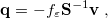$\begin{equation} \label{eq:C-PCM} \mathbf{q} = -f_\varepsilon \mathbf{S}^{-1}\mathbf{v} \; , \end{equation}$

(11.13)

and as discussed in Section 11.2.3 the user has the option to choose either the original value suggested by Klamt [583, 599], $f_\varepsilon = (\varepsilon -1)/(\varepsilon +1/2)$ , or else $f_\varepsilon = (\varepsilon -1)/\varepsilon$ as in, e.g., Refs. [584, 586, 593]. More importantly, however, COSMO differs from C-PCM in that the former includes a correction for outlying charge that goes beyond Eq. eq:C-PCM, whereas C-PCM consists of nothing more than induced surface charges computed (self-consistently) according to Eq. eq:C-PCM

Upon solution of Eq. eq:C-PCM, the outlying charge correction in COSMO [599, 600] is obtained by first defining a larger cavity that is likely to contain essentially all of the solute’s electron density; in practice, this typically means using atomic radii of 1.95 $R$ , where $R$ denotes the original atomic van der Waals radius that was used to compute $\mathbf{q}$ . (Note that unlike the PCMs described in Sections 11.2.2 and 11.2.3, where the atomic radii have default values but a high degree of user-controllability is allowed, the COSMO atomic radii are parameterized for this model and are fixed.) A new set of charges, 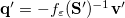$\mathbf{q}’ = -f_\varepsilon (\mathbf{S}’)^{-1}\mathbf{v}’$ , is then computed on this larger cavity surface, and the charges on the original cavity surface are adjusted to new values, $\mathbf{q}” = \mathbf{q}+\mathbf{q}’$ . Finally, a corrected electrostatic potential on the original surface is computed according to $\mathbf{v}” = -f_\varepsilon \mathbf{S}\mathbf{q}”$ . It is this potential that is used to compute the solute–continuum electrostatic interaction (polarization energy), $G_{\rm pol} = \tfrac {1}{2} \sum _ i q_ i” v_ i”$ . (For comparison, when the C-PCM approach described in Section 11.2.2 is used, the electrostatic polarization energy is $G_{\rm pol} = \tfrac {1}{2}\sum _ i q_ i^{} v_ i^{}$ , computed using the original surface charges $\mathbf{q}$ and surface electrostatic potential $\mathbf{v}$ .) With this outlying charge correction, Q-Chem’s implementation of COSMO resembles the one in Turbomole [640].

A COSMO calculation is requested by setting SOLVENT_METHOD = COSMO in the $rem section, in addition to normal job control variables. The keyword Dielectric in the $solvent section is used to set the solvent’s static dielectric constant, as described above for other solvation models. COSMO calculations can also be used as a starting point for “COSMO-RS” calculations [641, 609], where RS stands for “real solvent”. The COSMO-RS approach is not included in Q-Chem and requires the COSMOtherm program, which is licensed separately through COSMOlogic [610]. Q-Chem users who are interested in COSMOtherm can request special versions of Q-Chem for the generation of $\sigma$ -surface files that are needed by COSMOtherm.

11.2.7 SM $x$ Models

The SM $x$ models developed by Cramer, Truhlar, and co-workers at the University of Minnesota are a class of implicit solvation models that are designed to be “universal” in the sense that they can be applied to any solvent for which a small of descriptors is known [606]. (Note that the $x$ in SM $x$ is simply a version number; versions SM8 and SM12 are available in Q-Chem.) In particular, the solvent descriptors are:

dielectric constant
refractive index
bulk surface tension
acidity on the Abraham scale
basicity on the Abraham scale
carbon aromaticity, which equals the fraction of non-hydrogenic solvent atoms that are aromatic carbon atoms
electronegative halogenicity, which equals the fraction of non-hydrogenic solvent atoms that are F, Cl, or Br).

These models consist of a generalized Born treatment of continuum electrostatic interactions, along with non-electrostatic interactions that are parameterized in terms of atomic surface tensions. The non-electrostatic interactions include cavitation, dispersion, and changes in solvent structure, and the treatment of these non-electrostatic effects is crucial to obtaining accurate (free) energies of solvation.

11.2.7.1 The SM8 Model

The SM8 model is described in detail in Ref. Marenich:2007. It may be employed in conjunction with density functional theory (with any density functional available in Q-Chem) or with Hartree-Fock theory, but is intended for use only with the 6-31G*, 6-31+G*, and 6-31+G** basis sets, for reasons discussed below.

Bulk (continuum) electrostatic interactions in SM8 are described in terms of a generalized Born (GB) SCRF, using a solute cavity constructed from atom-centered spheres. For the atoms H, C, N, O, F, Si, P, S, Cl, and Br, atomic radii have been specifically optimized for use with SM8, whereas for other atoms the Bondi radius is used [619], or else a value of 2.0 for atoms not included in Bondi’s paper. Geometry-dependent radii are computed from these “intrinsic” Coulomb radii via a de-screening approximation [597].

In addition to GB electrostatics, there are several other contributions to the SM8 standard-state free energy of solvation. The first of these is called the electronic-nuclear-polarization (ENP) energy, or simply the electronic polarization (EP) energy if the solute geometry is assumed to be identical in the gas and solution phases. Another contribution to the free energy of solvation comes from short-range interactions with solvent molecules in the first solvation shell, and is sometimes called the cavitation/dispersion/solvent-structure (CDS) term. The CDS contribution to the solvation energy is a sum of terms that are each proportional (with geometry-dependent proportionality constants called atomic surface tensions) to the solvent-accessible surface areas (SASAs) of the individual solute atoms. The SASA of the solute molecule is the area of a surface generated by the center of a spherical effective solvent molecule rolling on the van der Waals surface of the solute molecule, as in the solvent-accessible surface that was mentioned in Section 11.2.2. The SASA is computed using the Analytic Surface Area (ASA) algorithm of Ref. [642] and Bondi’s values for the van der Waals radii [619], or else a value of 2.0 if no Bondi radius is available. (Note that, as in the case of non-electrostatic interactions in PCMs, this means that a different molecular surface is used for the bulk electrostatics as compared to the non-electrostatic interactions.) The solvent probe radius used to generate the SASAs is set to 0.40 for all solvents. Note that the solvent-structure part of the CDS term includes many aspects of solvent structure that are not described by bulk electrostatics, for example, hydrogen bonding, exchange repulsion, and the variation of the effective dielectric constant in the first solvation shell, relative to its bulk value. The semi-empirical nature of the CDS term also makes up for errors due to ( $i$ ) assuming fixed and model-dependent values of the intrinsic Coulomb radii, and ( $ii$ ) any systematic errors in the description of the solute–solvent electrostatic interactions using the GB approximation.

The final component of the SM8 solvation free energy is the concentration component. This is zero if the standard-state concentration of the solute is the same in the gas and solution phases (e.g., if it is 1 mole/liter in the gas phase as well as in the solution). Otherwise, this correction can be computed using ideal gas formulas, as discussed below.

SM8 does not require the user to assign molecular mechanics atom types to atoms or groups; all atomic surface tensions in the theory are unique and continuous functions of the solute geometry, defined by the model and calculated internally within Q-Chem. In principle, SM8 can be used with any level of electronic structure theory so long as accurate partial charges can be computed, but Q-Chem’s implementation of SM8 specifically uses self-consistently polarized Charge Model 4 (CM4) class IV charges [643] CM4 charges are obtained from Löwdin population analysis charges, via a mapping whose parameters depend on the basis set (and only on the basis set, not on the density functional or anything else). Basis sets supported for SM8 calculations in Q-Chem are:

6-31G*
6-31+G*
6-31+G**

The charge mapping parameters are given in Ref. Kelly:2005. Other basis sets should not be used in SM8 calculations.

The SM8 solvation free energy is output at $T=298$ K for a standard-state concentration of 1 M in both the gas and solution phase. However, solvation free energies in the literature are often tabulated using a standard state of $P=1$ atm for the gase. To convert 1 M-to1 M solvation free energies at 298 K to a standard state consisting of $P=1$ atm for the gas and a 1 M concentration in solution, add $+1.89$ kcal/mol to the computed solvation free energy.

Solution-phase geometry optimizations can be carried out, but basis sets that use spherical harmonic $d$ functions, or angular momentum higher than $d$ ( $f$ , $g$ , etc..) are not supported. Since, by definition, the 6-31G*, 6-31+G*, and 6-31+G** basis sets have Cartesian $d$ shells, they are examples of basis sets that may be used for geometry optimization with SM8. Solution-phase Hessian calculations can be carried out by numerical differentiation of analytical energy gradients or by double differentiation of energies, although the former procedure is both more stable and more economical. The analytic gradients of SM8 are based on the analytical derivatives of the polarization free energy and the analytical derivatives of the CDS terms derived in Ref. Zhu:1999.

An SM8 calculation is requested by setting SOLVENT_METHOD = SM8 in the $rem section, along with other job-control variables appropriate for a Hartree-Fock or DFT calculation. Additional variables for SM $x$ calculations should be listed in a $smx input section; for SM8, the only additional variable that is required is the name of the solvent:

Solvent

Sets the SM $x$ solvent

INPUT SECTION: $smx
TYPE:

STRING

DEFAULT:

water

OPTIONS:

Any name from the list of solvents given below.

RECOMMENDATION:

NONE

1,1,1-trichloroethane	bromoethane	$m$ -ethylbenzoate
1,1,2-trichloroethane	bromooctane	$m$ -ethylethanoate
1,1-dichloroethane	butanal	$m$ -ethylmethanoate
1,2,4-trimethylbenzene	butanoicacid	$m$ -ethylphenylketone
1,4-dioxane	butanone	$m$ -ethylpropanoate
1-bromo-2-methylpropane	butanonitrile	$m$ -ethylbutanoate
1-bromopentane	butylethanoate	$m$ -ethylcyclohexane
1-bromopropane	butylamine	$m$ -ethylformamide
1-butanol	butylbenzene	$m$ -xylene
1-chloropentane	carbon disulfide	heptane
1-chloropropane	carbon tetrachloride	hexadecane
1-decanol	chlorobenzene	hexane
1-fluorooctane	chlorotoluene	nitrobenzene
1-heptanol	$cis$ -1,2-dimethylcyclohexane	nitroethane
1-hexanol	decalin	nitromethane
1-hexene	cyclohexane	methylaniline
1-hexyne	cyclohexanone	nonane
1-iodobutane	cyclopentane	octane
1-iodopentene	cyclopentanol	pentane
1-iodopropane	cyclopentanone	$o$ -chlorotoluene
1-nitropropane	decane	$o$ -cresol
1-nonanol	dibromomethane	$o$ -dichlorobenzene
1-octanol	dibutyl ether	$o$ -nitrotoluene
1-pentanol	dichloromethane	$o$ -xylene
1-pentene	diethyl ether	pentadecane
1-pentyne	diethylsulfide	pentanal
1-propanol	diethylamine	pentanoic acid
2,2,20trifluoroethanol	diiodomethane	pentylethanoate
2,2,4-trimethylpentane	dimethyldisulfide	pentylamine
2,4-dimethylpentane	dimethylacetamide	perfluorobenzene
2,4-dimethylpyridine	dimethylformamide	phenyl ether
2,6-dimethylpyridine	dimethylpyridine	propanal
2-bromopropane	dimethyl sulfoxide	propanoic acid
2-chlorobutane	dipropylamine	propanonitrile
2-heptanone	dodecane	propylethanoate
2-hexanone	$E$ -1,2-dichloroethene	propylamine
2-methylpentane	$E$ -2-pentene	$p$ -xylene
2-methylpyridine	ethanethiol	pyridine
2-nitropropane	ethanol	pyrrolidine
2-octanone	ethylethanoate	$sec$ -butanol
2-pentanone	ethylmethanoate	$t$ -butanol
2-propanol	ethylphenyl ether	$t$ -butylbenzene
2-propen-1-ol	ethylbenzene	tetrachloroethene
3-methylpyridine	ethylene glycol	tetrahydrofuran
3-pentanone	fluorobenzene	tetrahyrothiophenedioxide
4-heptanone	formamide	tetralin
4-methyl-2-pentanone	formic acid	thiophene
4-methylpyridine	hexadecyliodide	thiophenol
5-nonanone	hexanoic acid	toluene
acetic acid	iodobenzene	$trans$ -decalin
acetone	iodoethane	tribromomethane
acetonitrile	iodomethane	tributylphosphate
aniline	isobutanol	trichloroethene
anisole	isopropyl ether	trichloromethane
benzaldehyde	isopropylbenzene	triethylamine
benzene	isopropyltoluene	undecane
benzonitrile	$m$ -cresol	water
benzyl alcohol	mesitylene	$Z$ -1,2-dichloroethene
bromobenzene	methanol	other

The final choice, Solvent = “other”, requires an additional free-format file called “solvent_data” that should contain the float-point values of the following solvent descriptors:

Dielec	dielectric constant, $\epsilon$ , of the solvent
SolN	index of refraction at optical frequencies at 293 K, $n_{20}^{D}$
SolA	Abraham’s hydrogen bond acidity, $\sum {\alpha }_2^{H}$
SolB	Abraham’s hydrogen bond basicity, $\sum {\beta }_2^{H}$
SolG	$\gamma = \gamma _ m / \gamma ^{0}$ (default is 0.0), where $\gamma _ m$ is the macroscopic surface tension at air/solvent
	interface at 298 K, and $\gamma ^{0}$ is 1 $cal~ mol^{-1}~ {\AA }^{-2}$ (1 dyne/cm = 1.43932 cal mol $^{-1}$ $^{-2}$ )
SolC	aromaticity, $\phi$ : the fraction of non-hydrogenic solvent atoms that are aromatic
	carbon atoms
SolH	electronegative “halogenicity”, $\psi$ : the fraction of non-hydrogenic solvent atoms that are
	F, Cl or Br

For a desired solvent, these values can be derived from experiment or from interpolation or extrapolation of data available for other solvents. Solvent parameters for common organic solvents are tabulated in the Minnesota Solvent Descriptor Database. The latest version of this database is available at:

http://comp.chem.umn.edu/solvation/mnsddb.pdf

The SM8 test suite contains the following representative examples:

single-point solvation energy and analytical gradient calculation for 2,2-dichloroethenyl dimethyl phosphate in water at the M06-2X/6-31G* level;
single-point solvation energy calculation for 2,2-dichloroethenyl dimethyl phosphate in benzene at the M06-2X/6-31G* level;
single-point solvation energy calculation for 2,2-dichloroethenyl dimethyl phosphate in ethanol at the M06-2X/6-31G* level;
single-point solvation energy calculation for 5-fluorouracil in water at the M06/6-31+G* level;
single-point solvation energy calculation for 5-fluorouracil in octanol at the M06-L/6-31+G* level;
single-point solvation energy and analytical gradient calculation for 5-fluorouracil in fluorobenzene at the M06-HF/6-31+G** level;
geometry optimization for protonated methanol $\rm CH_3OH_2^+$ in water at the B3LYP/6-31G* level;
finite-difference frequency (with analytical gradient) calculation for protonated methanol $\rm CH_3OH_2^+$ in water at the B3LYP/6-31G* level.

Users who wish to calculate solubilities can calculate them from the free energies of solvation by the method described in Ref. Thompson:2003. The present model can also be used with confidence to calculate partition coefficients (e.g., Henry’s Law constants, octanol/water partition coefficients, etc..) by the method described in Ref. Cramer:2001.

The user should note that the free energies of solvation calculated by the SM8 model in the current version of Q-Chem are all what may be called equilibrium free energies of solvation. The non-equilibrium algorithm required for vertical excitation energies [647] is not yet available in Q-Chem.

11.2.7.2 The SM12 Model

The SM12 model [598] is also available in Q-Chem. Similar to SM8, it employs (a) the generalized Born approximation for the bulk electrostatic contribution to the free energy of solvation, and (b) the same formulas (with re-optimized parameters) for CDS contributions. SM12 holds several advantages over SM8, and perhaps foremost among these is that it uses CM5 charges [459], which are based on Hirshfeld population analysis, or else charges derived from the electrostatic potential [648, 455], for the bulk electrostatics term. These charges are stable with respect to extension of the basis set, and thus SM12 can be used with larger basis sets whereas SM8 is limited to 6-31G*, 6-31+G*, and 6-31+G**, due to instabilities in the Löwdin charges in larger basis sets. In addition, SM12 is parameterized using a more diverse training set as compared to SM8, and is defined for the entire periodic table. However, the SM12 analytic gradient is not available in Q-Chem at present.

An SM12 calculation is requested by setting SOLVENT_METHOD = SM12 in the $rem section. The manner in which the electrostatic term is computed is controlled by the Charges keyword in the $smx input section.

Charges

Sets the type of atomic charges for the SM12 electrostatic term.

INPUT SECTION: $smx
TYPE:

STRING

DEFAULT:

CM5

OPTIONS:

CM5

Charge Model 5 charges [459]

MK

Merz-Singh-Kollman charges [648]

CHELPG

ChElPG charges [455]

RECOMMENDATION:

None. Merz-Singh-Kollman and ChElPG charges are fit to reproduce the molecular electrostatic potential on the van der Waals surface or on a cubic grid, respectively, whereas CM5 is an empirical model based on Hirshfeld population analysis.

Example 11.250 SM12CM5 calculation of the solvation free energy of water in the 1-octanol solvent.

$molecule
0 1
O   0.000000  0.125787   0.000000
H   0.758502  -0.503148  0.000000
H  -0.758502  -0.503148  0.000000
$end

$rem
jobtype sp
scf_guess core
method b3lyp
basis 6-31G*
sym_ignore true
solvent_method sm12
$end

$smx
solvent 1octanol
charges chelpg
$end

11.2.8 Langevin Dipoles Solvation Model

Q-Chem provides the option to calculate molecular properties in aqueous solution and the magnitudes of the hydration free energies by the Langevin dipoles (LD) solvation model developed by Jan Florián and Arieh Warshel [595, 596] at the University of Southern California. In this model, a solute molecule is surrounded by a sphere of point dipoles, with centers on a cubic lattice. Each of these “Langevin” dipoles changes its size and orientation in the electrostatic field of the solute and the other Langevin dipoles. The electrostatic field from the solute is determined rigorously by the integration of its charge density, whereas for dipole–dipole interactions, a 12 cutoff is used. The Q-Chem/ChemSol 1.0 implementation of the LD model is fully self-consistent in that the molecular quantum mechanical calculation takes into account solute–solvent interactions. Further details on the implementation and parameterization of this model can be found in the original literature [595, 596].

The results of ChemSol calculations are printed in the standard output file. Below is a part of the output for a calculation on the methoxide anion (corresponding to the sample input given later on, and the sample file in the $QC/samples directory).

Energy Component	Value / kcal mol $^{-1}$
LD Electrostatic energy	$-86.14$
Hydrophobic energy	0.28
van der Waals energy	$-1.95$
Bulk correction	$-10.07$
Solvation free energy, $\Delta G$ (ILD)	$-97.87$

Table 11.3: Results of the iterative Langevin Dipoles (ILD) solvation model, for aqueous methoxide.

The total hydration free energy, $\Delta G$ (ILD) is calculated as a sum of several contributions. Note that the electrostatic part of $\Delta G$ is calculated by using the linear-response approximation [595] and contains contributions from the polarization of the solute charge distribution due to its interaction with the solvent. This results from the self-consistent implementation of the Langevin dipoles model within Q-Chem.

To perform an LD calculation in Q-Chem, specify normal job-control variables for a Hartree-Fock or DFT calculation, and set SOLVENT_METHOD = CHEM_SOL in the $rem section. Additional fine-tuning is accomplished using a set of keywords in a $chem_sol input section. The remainder of this section summarizes these keywords.

EField

Determines how the solute charge distribution is approximated in evaluating the electrostatic field of the solute.

INPUT SECTION: $chemsol
TYPE:

INTEGER

DEFAULT:

1

OPTIONS:

1

Exact solute charge distribution is used.

0

Solute charge distribution is approximated by Mulliken atomic charges.

RECOMMENDATION:

None. The Mulliken-based procedure is faster but less rigorous.

NGrids

Sets the number of grids used to calculate the average hydration free energy.

INPUT SECTION: $chemsol
TYPE:

INTEGER

DEFAULT:

5

$\Delta G_{\ensuremath{\mathrm{hydr}}}$ will be averaged over 5 different grids.

OPTIONS:

$n$

Use $n$ different grids.

RECOMMENDATION:

None. The maximum allowed value of $n$ is 20.

Print

Controls printing in the ChemSol part of the Q-Chem output file.

INPUT SECTION: $chemsol
TYPE:

INTEGER

DEFAULT:

0

OPTIONS:

0

Limited printout

1

Full printout

RECOMMENDATION:

None.

Accurate calculations of hydration free energies require a judicious choice of the solute–solvent boundary in terms of atom-type dependent parameters. The default atomic van der Waals radii available in Q-Chem were chosen to provide reasonable hydration free energies for most solutes and basis sets. These parameters basically coincide with the ChemSol 2.0 radii given in Ref. Florian:1999. The only difference between the Q-Chem and ChemSol 2.0 atomic radii stems from the fact that Q-Chem parameter set uses radii for carbon and oxygen that are independent of the atom’s hybridization state. User-defined atomic radii can be specified by declaring the option ReadRadii in the $chem_sol input section, and then placing the radii in the $van_der_waals section. Two different (and mutually exclusive) formats can be used, as shown below.

$van_der_waals
1
atomic_number   vdW_radius
...
$end

$van_der_waals
2
sequential_atom_number   vdW_radius 
...
$end

The purpose of the second format is to permit the user to customize the radius of specific atoms, in the order that they appear in the $molecule section, rather than simply by atomic numbers as in format 1. The radii of atoms that are not listed in the $van_der_waals input will be assigned default values. The atomic radii that were used in the calculation are printed in the ChemSol part of the output file in the column denoted rp. All radii should be given in Angstroms.

Example 11.251 A Langevin dipoles calculation on the methoxide anion. A customized value is specified for the radius of the C atom.

$molecule
  -1  1
   C   0.0000   0.0000  -0.5274
   O   0.0000   0.0000   0.7831
   H   0.0000   1.0140  -1.0335
   H   0.8782  -0.5070  -1.0335
   H  -0.8782  -0.5070  -1.0335
$end

$rem
   METHOD            hf
   BASIS             6-31G
   SCF_CONVERGENCE   6
   SOLVENT_METHOD    Chem_Sol
$end

$chemsol
ReadRadii
$end

$van_der_waals
2
1 2.5
$end

0	Do not use a solvation model.
ONSAGER	Use the Kirkwood-Onsager model (Section 11.2.1).
PCM	Use an apparent surface charge, polarizable continuum model
	(Section 11.2.2).
ISOSVP	Use the iso-density implementation of the SS(V)PE model
	(Section 11.2.5).
COSMO	Use COSMO (similar to C-PCM but with an outlying charge
	correction [599, 600]; see Section 11.2.6).
SM8	Use version 8 of the Cramer-Truhlar SM $x$ model (Section 11.2.7.1).
SM12	Use version 12 of the SM $x$ model (Section 11.2.7.2).
CHEM_SOL	Use the Langevin Dipoles model (Section 11.2.8).

CPCM	Conductor-like PCM with $f_\varepsilon = (\varepsilon -1)/\varepsilon$ .
COSMO	Original conductor-like screening model with $f_\varepsilon = (\varepsilon -1)/(\varepsilon +1/2)$ .
IEFPCM	IEF-PCM with an asymmetric $\mathbf{K}$ matrix.
SSVPE	SS(V)PE model, equivalent to IEF-PCM with a symmetric $\mathbf{K}$ matrix.

SWIG	Switching/Gaussian method
ISWIG	“Improved” Switching/Gaussian method with an alternative switching function
Spherical	Use a single, fixed sphere for the cavity surface.
Fixed	Use discretization point charges instead of smooth Gaussians.

BONDI	Use the (extended) set of Bondi radii.
FF	Use Lennard-Jones radii from a molecular mechanics force field.
UFF	Use radii form the Universal Force Field.
READ	Read the atomic radii from a $van_der_waals input section.

0	Prints PCM energy and basic surface grid information. Minimal additional printing.
1	Level 0 plus PCM solute-solvent interaction energy components and Gauss’ Law error.
2	Level 1 plus surface grid switching parameters and a `.PQR` file for visualization of
	the cavity surface apparent surface charges.
3	Level 2 plus a `.PQR` file for visualization of the electrostatic potential at the surface
	grid created by the converged solute.
4	Level 3 plus additional surface grid information, electrostatic potential and apparent
	surface charges on each SCF cycle.
5	Level 4 plus extensive debugging information.

Cav	Cavitation energy
Buck	Buckingham dispersion and repulsion energy from atomic number
LJ	Lennard-Jones dispersion and repulsion energy from force field
BuckCav	Buck + Cav
LJCav	LJ + Cav

Input (TYPE)	Description
Number1 (INTEGER):	The atomic number of the atom
Number2 (INTEGER):	How many of this atom are in a solvent molecule
Number3 (INTEGER):	Force field atom type
SASrad (FLOAT):	Probe radius (in ) for defining the solvent accessible surface

Marcus	Do slow-fast charge separation in the ground state.
Excited	Do slow-fast charge separation in an excited-state.

Ground	Run self-consistent SS method in the ground-state with a given slow polarization charges.
Perturb	Perform ptSS and ptLR for vertical excitations.
$i$	The $i$ -th excited-state used for charge separation (for emission).

INVERSION	Direct matrix inversion
CG	Iterative conjugate gradient

0	Turns off matrix decomposition
1	Turns on matrix decomposition
3	Option 1 plus only stores upper half of matrix and enhances gradient evaluation

0	runs a gas-phase calculation and after
	convergence runs the SS(V)PE computation.
1	does not run a gas-phase calculation.

0	No guessing.
1	Read a guess from a previous Q-Chem solvation computation.
2	Use a guess specified by the $svpirf section from the input

0	use the electronic iso-density surface.
1	use a spherical cavity surface.

0	Single center Lebedev integration.
1	Single center spherical polar integration.

Valid choices are:	6, 18, 26, 38, 50, 86, 110, 146, 170, 194, 302, 350, 434, 590, 770,
	974, 1202, 1454, 1730, 2030, 2354, 2702, 3074, 3470, 3890, 4334,
	4802, or 5294.

0	use LU decomposition in memory if space permits, else switch to LINEQ=2
1	use conjugate gradient iterations in memory if space permits, else use LINEQ=2
2	use conjugate gradient iterations with the system matrix stored externally on disk.

0	No translation (i.e., center of the cavity at the origin
	of the atomic coordinate system)
1	Translate to the center of nuclear mass.
2	Translate to the center of nuclear charge.
3	Translate to the midpoint of the outermost atoms.
4	Translate to midpoint of the outermost non-hydrogen atoms.
5	Translate to user-specified coordinates in Bohr.
6	Translate to user-specified coordinates in Angstroms.

0	No rotation.
1	Rotate initial $xyz$ axes of the integration grid to coincide
	with principal moments of nuclear inertia (relevant if ITRNGR=1)
2	Rotate initial $xyz$ axes of integration grid to coincide with
	principal moments of nuclear charge (relevant if ITRNGR=2)
3	Rotate initial $xyz$ axes of the integration grid through user-specified
	Euler angles as defined by Wilson, Decius, and Cross.

0	no cavity check, use only the outer cavity
1	cavity check, generating both the inner and outer cavities and compare.