10.2 Wavefunction Analysis
Q-Chem performs a number of standard wavefunction analyses by default. Switching the $rem variable WAVEFUNCTION_ANALYSIS to FALSE will prevent the calculation of all wavefunction analysis features (described in this section). Alternatively, each wavefunction analysis feature may be controlled by its $rem variable. (The NBO package which is interfaced with Q-Chem is capable of performing more sophisticated analyses. See later in this chapter and the NBO manual for details).
WAVEFUNCTION_ANALYSIS
Controls the running of the default wavefunction analysis tasks.
TYPE:
LOGICAL
DEFAULT:
TRUE
OPTIONS:
TRUE
Perform default wavefunction analysis.
FALSE
Do not perform default wavefunction analysis.
RECOMMENDATION:
None
Note: WAVEFUNCTION_ANALYSIS has no effect on NBO, solvent models or vibrational analyses.
10.2.1 Population Analysis
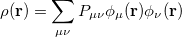
The one-electron charge density, usually written as
 |
(10.1) |
represents the probability of finding an electron at the point  , but implies little regarding the number of electrons associated with a given nucleus in a molecule. However, since the number of electrons
  is related to the occupied orbitals
  by
by
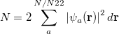 |
(10.2) |
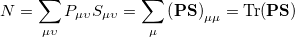
We can substitute the atomic orbital (AO) basis expansion of  into Eq. (10.2) to obtain
 |
(10.3) |
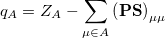
where we interpret  as the number of electrons associated with
  . If the basis functions are atom-centered, the number of electrons associated with a given atom can be obtained by summing over all the basis functions. This leads to the Mulliken formula for the net charge of the atom
  :
:
 |
(10.4) |
where  is the atom’s nuclear charge. This is called a Mulliken population analysis [9]. Q-Chem performs a Mulliken population analysis by default.
POP_MULLIKEN
Controls running of Mulliken population analysis.
TYPE:
LOGICAL/INTEGER
DEFAULT:
TRUE
(or 1)
OPTIONS:
FALSE
(or 0) Do not calculate Mulliken Population.
TRUE
(or 1) Calculate Mulliken population
2
Also calculate shell populations for each occupied orbital.

Calculate Mulliken charges for both the ground state and any CIS,
RPA, or TDDFT excited states.
RECOMMENDATION:
Leave as TRUE, unless excited-state charges are desired. Mulliken analysis is a trivial additional calculation, for ground or excited states.
LOWDIN_POPULATION
Run a Löwdin population analysis instead of a Mulliken.
TYPE:
LOGICAL
DEFAULT:
FALSE
OPTIONS:
FALSE
Do not calculate Löwdin Populations.
TRUE
Run Löwdin Population analyses instead of Mulliken.
RECOMMENDATION:
None
Although conceptually simple, Mulliken population analyses suffer from a heavy dependence on the basis set used, as well as the possibility of producing unphysical negative numbers of electrons. An alternative is that of Löwdin Population analysis [454], which uses the Löwdin symmetrically orthogonalized basis set (which is still atom-tagged) to assign the electron density. This shows a reduced basis set dependence, but maintains the same essential features.
While Mulliken and Löwdin population analyses are commonly employed, and can be used to produce information about changes in electron density and also localized spin polarizations, they should not be interpreted as oxidation states of the atoms in the system. For such information we would recommend a bonding analysis technique (LOBA or NBO).
A more stable alternative to Mulliken or Löwdin charges are the so-called “CHELPG” charges (“Charges from the Electrostatic Potential on a Grid”) [455]. These are the atom-centered charges that provide the best fit to the molecular electrostatic potential, evaluated on a real-space grid outside of the van der Waals region and subject to the constraint that the sum of the CHELPG charges must equal the molecular charge. Q-Chem’s implementation of the CHELPG algorithm differs slightly from the one originally algorithm described by Breneman and Wiberg [455], in that Q-Chem weights the grid points with a smoothing function to ensure that the CHELPG charges vary continuously as the nuclei are displaced [456]. (For any particular geometry, however, numerical values of the charges are quite similar to those obtained using the original algorithm.) Note, however, that the Breneman-Wiberg approach uses a Cartesian grid and becomes expensive for large systems. (It is especially expensive when CHELPG charges are used in QM/MM-Ewald calculations [457].) For that reason, an alternative procedure based on atom-centered Lebedev grids is also available [457], which provides very similar charges using far fewer grid points. In order to use the Lebedev grid implementation the $rem variables CHELPG_H and CHELPG_HA must be set, which specify the number of Lebedev grid points for the hydrogen atoms and the heavy atoms, respectively.
CHELPG
Controls the calculation of CHELPG charges.
TYPE:
LOGICAL
DEFAULT:
FALSE
OPTIONS:
FALSE
Do not calculate CHELPG charges.
TRUE
Compute CHELPG charges.
RECOMMENDATION:
Set to TRUE if desired. For large molecules, there is some overhead associated with computing CHELPG charges, especially if the number of grid points is large.
CHELPG_HEAD
Sets the “head space” [455] (radial extent) of the CHELPG grid.
TYPE:
INTEGER
DEFAULT:
30
OPTIONS:
Corresponding to a head space of
, in .
RECOMMENDATION:
Use the default, which is the value recommended by Breneman and Wiberg [455].
CHELPG_DX
Sets the rectangular grid spacing for the traditional Cartesian CHELPG grid or the spacing between concentric Lebedev shells (when the variables CHELPG_HA and CHELPG_H are specified as well).
TYPE:
INTEGER
DEFAULT:
6
OPTIONS:
Corresponding to a grid space of
, in .
RECOMMENDATION:
Use the default (which corresponds to the “dense grid” of Breneman and Wiberg [455]), unless the cost is prohibitive, in which case a larger value can be selected. Note that this default value is set with the Cartesian grid in mind and not the Lebedev grid. In the Lebedev case, a larger value can typically be used.
CHELPG_H
Sets the Lebedev grid to use for hydrogen atoms.
TYPE:
INTEGER
DEFAULT:
NONE
OPTIONS:
Corresponding to a number of points in a Lebedev grid.
RECOMMENDATION:
CHELPG_H must always be less than or equal to CHELPG_HA. If it is greater, it will automatically be set to the value of CHELPG_HA.
CHELPG_HA
Sets the Lebedev grid to use for non-hydrogen atoms.
TYPE:
INTEGER
DEFAULT:
NONE
OPTIONS:
Corresponding to a number of points in a Lebedev grid (see Section 4.3.14.
RECOMMENDATION:
None.
Finally, Hirschfeld population analysis [458] provides yet another definition of atomic charges in molecules via a Stockholder prescription. The charge on atom ,  , is defined by
 |
(10.5) |
where is the nuclear charge of ,  is the isolated ground-state atomic density of atom
  , and
, and  is the molecular density. The sum goes over all atoms in the molecule. Thus computing Hirshfeld charges requires a self-consistent calculation of the isolated atomic densities (the promolecule) as well as the total molecule. Following SCF completion, the Hirshfeld analysis proceeds by running another SCF calculation to obtain the atomic densities. Next numerical quadrature is used to evaluate the integral in Eq. (10.5). Neutral ground-state atoms are used, and the choice of appropriate reference for a charged molecule is ambiguous (such jobs will crash). As numerical integration (with default quadrature grid) is used, charges may not sum precisely to zero. A larger XC_GRID may be used to improve the accuracy of the integration.
The charges (and corresponding molecular dipole moments) obtained using Hirshfeld charges are typically underestimated as compared to other charge schemes or experimental data. To correct this, Marenich et al. [459] introduced “Charge Model 5” (CM5), which employs a single set of parameters to map the Hirshfeld charges onto a more reasonable representation of the electrostatic potential. CM5 charges generally lead to more accurate dipole moments as compared to the original Hirshfeld charges, at negligible additional cost. CM5 is available for molecules composed of elements H–Ca, Zn, Ge–Br, and I.
The use of neutral ground-state atoms to define the promolecular density in Hirshfeld scheme has no strict theoretical basis and there is no unique way to construct the promolecular densities. For example, Li F, Li
F, Li F
F , or LiF could each be used to construct the promolecular densities for LiF. Furthermore, the choice of appropriate reference for a charged molecule is ambiguous, and for this reason Hirshfeld analysis is disable in Q-Chem for any molecule with a net charge. A solution for charged molecules is to use the iterative “Hirshfeld-I” partitioning scheme proposed by Bultinck et al. [460, 461], in which the reference state is not predefined but rather determined self-consistently, thus eliminating the arbitrariness. The final self-consistent reference state for Hirshfeld-I partitioning usually consists of non-integer atomic populations.
In the first iteration, the Hirshfeld-I method uses neutral atomic densities (as in the original Hirshfeld scheme),  with electronic population
  . This affords charges
 |
(10.6) |
on the first iteration. The new electronic population (number of electrons) for atom  is
is  , and is derived from the promolecular populations
  . One then computes new isolated atomic densities with
  and uses them to construct the promolecular densities in the next iteration. In general, the new weighting function for atom in the
  th iteration is
 |
(10.7) |
The atomic densities  with corresponding fractional electron numbers
  are obtained by linear interpolation between
  and
and  of the same atom [460, 462]:
 |
(10.8) |
where  and
and  denote the integers that bracket
  The two atomic densities on the right side of Eq. eq:interpolate are obtained from densities
  that are computed in advance. (That is, the method uses the neutral atomic density along with the densities for the singly- and doubly-charged cations and anions of the element in equation.) The Hirshfeld-I iterations are converged once the atomic populations change insignificantly between iterations, say
  [460, 463].
The iterative Hirshfeld scheme generally affords more reasonable charges as compared to the original Hirshfeld scheme. In LiF, for example, the original Hirshfeld scheme predicts atomic charges of  0.57 while the iterative scheme increases these charges to 0.93. The integral in Eq. eq:hirshc is evaluated by numerical quadrature, and the cost of each iteration of Hirshfeld-I is equal to the cost of computing the original Hirshfeld charges. Within Q-Chem, Hirshfeld-I charges are available for molecules containing only H, Li, C, N, O, F, S, and Cl. The $rem variable SYM_IGNORE must be set to TRUE for Hirshfeld-I analysis.
HIRSHFELD
Controls running of Hirshfeld population analysis.
TYPE:
LOGICAL
DEFAULT:
FALSE
OPTIONS:
TRUE
Calculate Hirshfeld populations.
FALSE
Do not calculate Hirshfeld populations.
RECOMMENDATION:
None
HIRSHFELD_READ
Switch to force reading in of isolated atomic densities.
TYPE:
LOGICAL
DEFAULT:
FALSE
OPTIONS:
TRUE
Read in isolated atomic densities from previous Hirshfeld calculation from disk.
FALSE
Generate new isolated atomic densities.
RECOMMENDATION:
Use default unless system is large. Note, atoms should be in the same order with same basis set used as in the previous Hirshfeld calculation (although coordinates can change). The previous calculation should be run with the -save switch.
HIRSHFELD_SPHAVG
Controls whether atomic densities should be spherically averaged in pro-molecule.
TYPE:
LOGICAL
DEFAULT:
TRUE
OPTIONS:
TRUE
Spherically average atomic densities.
FALSE
Do not spherically average.
RECOMMENDATION:
Use default.
CM5
Controls running of CM5 population analysis.
TYPE:
LOGICAL
DEFAULT:
FALSE
OPTIONS:
TRUE
Calculate CM5 populations.
FALSE
Do not calculate CM5 populations.
RECOMMENDATION:
None
HIRSHITER
Controls running of iterative Hirshfeld population analysis.
TYPE:
LOGICAL
DEFAULT:
FALSE
OPTIONS:
TRUE
Calculate iterative Hirshfeld populations.
FALSE
Do not calculate iterative Hirshfeld populations.
RECOMMENDATION:
None
HIRSHITER_THRESH
Controls the convergence criterion of iterative Hirshfeld population analysis.
TYPE:
INTEGER
DEFAULT:
5
OPTIONS:

Corresponding to the convergence criterion of
, in
.
RECOMMENDATION:
Use the default, which is the value recommended in Ref. Bultinck:2007
10.2.2 Examples
The iterative Hirshfeld population analysis for  .
.
$molecule
-1  1
 O     1.197566    -0.108087     0.000000
 H     1.415397     0.827014     0.000000
 H     0.134830    -0.084378     0.000000
 F    -1.236389     0.012239     0.000000

$end

$rem
sym_ignore true
method B3LYP
basis 6-31G*
hirshiter  true
$end
The next section discusses how to compute arbitrary electrostatic multipole moments for an entire molecule, including both ground- and excited-state electron densities. Occasionally, however, it is useful to decompose the electronic part of the multipole moments into contributions from individual MOs. This decomposition is especially useful for systems containing unpaired electrons [464], where the first-order moments  ,
,  , and
, and  characterize the centroid (mean position) of the half-filled MO, and the second-order moments determine its radius of gyration,
  , which characterizes the size of the MO. Upon setting PRINT_RADII_GYRE = TRUE, Q-Chem will print out centroids and radii of gyration for each occupied MO and for the overall electron density. If CIS or TDDFT excited states are requested, then this keyword will also print out the centroids and radii of gyration for each excited-state electron density.
PRINT_RADII_GYRE
Controls printing of MO centroids and radii of gyration.
TYPE:
LOGICAL/INTEGER
DEFAULT:
FALSE
OPTIONS:
TRUE
(or 1) Print the centroid and radius of gyration for each occupied MO and each density.
2
Print centroids and radii of gyration for the virtual MOs as well.
FALSE
(or 0) Do not calculate these quantities.
RECOMMENDATION:
None
10.2.3 Multipole Moments
Q-Chem can compute Cartesian multipole moments of the charge density to arbitrary order, both for the ground state and for excited states calculated using the CIS or TDDFT methods.
MULTIPOLE_ORDER
Determines highest order of multipole moments to print if wavefunction analysis requested.
TYPE:
INTEGER
DEFAULT:
4
OPTIONS:

Calculate moments to
RECOMMENDATION:
Use default unless higher multipoles are required.
CIS_MOMENTS
Controls calculation of excited-state (CIS or TDDFT) multipole moments
TYPE:
LOGICAL/INTEGER
DEFAULT:
FALSE
(or 0)
OPTIONS:
FALSE
(or 0) Do not calculate excited-state moments.
TRUE
(or 1) Calculate moments for each excited state.
RECOMMENDATION:
Set to TRUE if excited-state moments are desired. (This is a trivial additional calculation.) The MULTIPOLE_ORDER controls how many multipole moments are printed.
10.2.4 Symmetry Decomposition
Q-Chem’s default is to write the SCF wavefunction molecular orbital symmetries and energies to the output file. If requested, a symmetry decomposition of the kinetic and nuclear attraction energies can also be calculated.
SYMMETRY_DECOMPOSITION
Determines symmetry decompositions to calculate.
TYPE:
INTEGER
DEFAULT:
1
OPTIONS:
0
No symmetry decomposition.
1
Calculate MO eigenvalues and symmetry (if available).
2
Perform symmetry decomposition of kinetic energy and nuclear attraction
matrices.
RECOMMENDATION:
None
10.2.5 Localized Orbital Bonding Analysis
Localized Orbital Bonding Analysis (LOBA) [322] is a technique developed by Dr. Alex Thom and Eric Sundstrom at Berkeley with Prof. Martin Head-Gordon. Inspired by the work of Rhee and Head-Gordon [465], it makes use of the fact that the post-SCF localized occupied orbitals of a system provide a large amount of information about the bonding in the system.
While the canonical Molecular Orbitals can provide information about local reactivity and ionization energies, their delocalized nature makes them rather uninformative when looking at the bonding in larger molecules. Localized orbitals in contrast provide a convenient way to visualize and account for electrons. Transformations of the orbitals within the occupied subspace do not alter the resultant density; if a density can be represented as orbitals localized on individual atoms, then those orbitals can be regarded as non-bonding. If a maximally localized set of orbitals still requires some to be delocalized between atoms, these can be regarded as bonding electrons. A simple example is that of He versus H. In the former, the delocalized
  and
and  canonical orbitals may be transformed into 1s orbitals on each He atom, and there is no bond between them. This is not possible for the H molecule, and so we can regard there being a bond between the atoms. In cases of multiple bonding, multiple delocalized orbitals are required.
While there are no absolute definitions of bonding and oxidation state, it has been shown that the localized orbitals match the chemically intuitive notions of core, non-bonded, single- and double-bonded electrons, etc.. By combining these localized orbitals with population analyses, LOBA allows the nature of the bonding within a molecule to be quickly determined.
In addition, it has been found that by counting localized electrons, the oxidation states of transition metals can be easily found. Owing to polarization caused by ligands, an upper threshold is applied, populations above which are regarded as “localized” on an atom, which has been calibrated to a range of transition metals, recovering standard oxidation states ranging from  II to VII.
LOBA
Specifies the methods to use for LOBA
TYPE:
INTEGER
DEFAULT:
00
OPTIONS:


specifies the localization method
0 Perform Boys localization.
1 Perform PM localization.
2 Perform ER localization.

specifies the population analysis method
0 Do not perform LOBA. This is the default.
1 Use Mulliken population analysis.
2 Use Löwdin population analysis.
RECOMMENDATION:
Boys Localization is the fastest. ER will require an auxiliary basis set.
LOBA 12 provides a reasonable speed/accuracy compromise.
LOBA_THRESH
Specifies the thresholds to use for LOBA
TYPE:
INTEGER
DEFAULT:
6015
OPTIONS:


specifies the threshold to use for localization

specifies the threshold to use for occupation
Both are measured in %
RECOMMENDATION:
Decrease
On a technical note, LOBA can function of both Restricted and Unrestricted SCF calculations. The figures printed in the bonding analysis count the number of electrons on each atom from that orbital (i.e., up to 1 for Unrestricted or singly occupied Restricted orbitals, and up to 2 for double occupied Restricted.)
10.2.6 Excited-State Analysis
For CIS, TDHF, and TDDFT excited-state calculations, we have already mentioned that Mulliken population analysis of the excited-state electron densities may be requested by setting POP_MULLIKEN = , and multipole moments of the excited-state densities will be generated if CIS_MOMENTS = TRUE. Another useful decomposition for excited states is to separate the excitation into “particle” and “hole” components, which can then be analyzed separately [329]. To do this, we define a density matrix for the excited electron,
 |
(10.9) |
and a density matrix for the hole that is left behind in the occupied space:
 |
(10.10) |
The quantities  and
and  are the transition density matrices, i.e., the components of the TDDFT eigenvector [466]. The indices and
  denote MOs that occupied in the ground state, whereas and index virtual MOs. Note also that
  , the difference between the ground- and excited-state density matrices.
Upon transforming  and
and  into the AO basis, one can write
 |
(10.11) |
where  is the total charge that is transferred from the occupied space to the virtual space. For a CIS calculation, or for TDDFT within the Tamm-Dancoff approximation [375],
  . For full TDDFT calculations, may be slightly different than .
Comparison of Eq. () to Eq. (10.3) suggests that the quantities  and
and  are amenable to to population analyses of precisely the same sort used to analyze the ground-state density matrix. In particular,
  represents the
  th AO’s contribution to the excited electron, while
  is a contribution to the hole. The sum of these quantities,
 |
(10.12) |
represents the contribution to arising from the th AO. For the particle/hole density matrices, both Mulliken and Löwdin population analyses available, and are requested by setting CIS_MULLIKEN = TRUE.
CIS_MULLIKEN
Controls Mulliken and Löwdin population analyses for excited-state particle and hole density matrices.
TYPE:
LOGICAL/INTEGER
DEFAULT:
FALSE
OPTIONS:
FALSE
(or 0) Do not perform particle/hole population analysis.
TRUE
(or 1) Perform both Mulliken and Löwdin analysis of the particle and hole
density matrices for each excited state.
RECOMMENDATION:
Set to TRUE if desired. This represents a trivial additional calculation.
Although the excited-state analysis features described in this section require very little computational effort, they are turned off by default, because they can generate a large amount of output, especially if a large number of excited states are requested. They can be turned on individually, or collectively by setting CIS_AMPL_ANAL = TRUE. This collective option also requests the calculation of natural transition orbitals (NTOs), which were introduced in Section 6.11.2. (NTOs can also be requested without excited-state population analysis. Some practical aspects of calculating and visualizing NTOs are discussed below, in Section 10.6.2.)
CIS_AMPL_ANAL
Perform additional analysis of CIS and TDDFT excitation amplitudes, including generation of natural transition orbitals, excited-state multipole moments, and Mulliken analysis of the excited state densities and particle/hole density matrices.
TYPE:
LOGICAL
DEFAULT:
FALSE
OPTIONS:
TRUE
Perform additional amplitude analysis.
FALSE
Do not perform additional analysis.
RECOMMENDATION:
None
10.2.7 Excited-State Analysis for Correlated Methods
For excited states calculated using CC/EOM-CC or ADC methods, there are also a number of excited-state analyses available. The analyses are based either on the transition densities or on the difference densities of the excited states. The transition density based analyses comprise the construction and export of natural transition orbitals (NTO), as well as electron and hole densities, the evaluation of charge transfer numbers, and an exciton analysis. Furthermore, the formation and export of state-averaged NTOs, and the decomposition of the excited states into transitions of state-averaged NTOs are implemented. The difference and/or state densities can be exported themselves, as well as employed to construct and export natural orbitals, natural difference orbitals, and attachment and detachment densities. In addition, a Mulliken or Loewdin population analysis and an exciton analysis can be performed based on the difference/state densities.
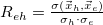
Details on the implemented excited-state analyses can be found in [467, 468, 469]. The main descriptors of the various analyses which are printed for each excited state are given below.
Transition density matrix analysis
Descriptor
Explanation
Leading SVs
Largest NTO occupation numbers
Sum of SVs
Sum of NTO occupation numbers
PR_NTO
NTO participation ratio

omega
Atomic charge transfer number

<r_h> [Ang]
Mean position of hole

<r_e> [Ang]
Mean position of electron

|<r_e - r_h>| [Ang]
Electron-hole distance
Hole size [Ang]
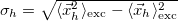
Electron size [Ang]
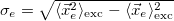
RMS electron-hole separation [Ang]
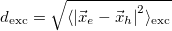
Covariance(r_h, r_e) [Ang^2]

Correlation coefficient
Difference/state density matrix analysis
Descriptor
Explanation
n_u and n_u,nl
Number of unpaired electrons
 and
and 
PR_NO
NO participation ratio

p_D and p_A
Number of de-/attached electrons
 and
and 
PR_D and PR_A
De- and attachment ratio
 and
and 
<r_h> [Ang]
Mean position of detachment density

<r_e> [Ang]
Mean position of attachment density

|<r_e - r_h>| [Ang]
Electron-hole distance
Hole size [Ang]
Variance of detachment density

Electron size [Ang]
Variance of attachment density

To activate any excited-state analysis STATE_ANALYSIS has to be set to TRUE. For individual analyses there is currently only a limited amount of fine grained control. The construction and export of any type of orbitals is controlled by MOLDEN_FORMAT to export the orbitals as MolDen files, and NTO_PAIRS which specifies the number of important orbitals to print. Setting MAKE_CUBE_FILES to TRUE triggers the construction and export of densities as “Cube” files (see 10.6.4 for details). Activating transition densities in $plots will generate “Cube” files for the transition density, the electron density, and the hole density of the respective excited states, while activating state densities or attachment/detachment densities will generate “Cube” files for the state density, the difference density, the attachment density and the detachment density. Please be aware that setting GUI=2 switches off the generation of “Cube” files. The population analyses are controlled by POP_MULLIKEN and LOWDIN_POPULATION. Setting the latter to TRUE will enforce Loewdin population analysis to be employed, while by default the Mulliken population analysis is used.
Any MolDen or “Cube” files generated by the excited state analyses can be found in the directory plots in the job’s scratch directory. Their names always start with a unique identifier of the excited state (the exact form of this human readable identifier varies with the excited state method). The names of MolDen files are then followed by either _no.mo, _ndo.mo, or _nto.mo depending on the type of orbitals they contain. In case of “Cube” files the state identifier is followed by _dens, _diff, _trans, _attach, _detach, _elec, or _hole for state, difference, transition, attachment, detachment, electron, or hole densities, respectively. All “Cube” files are suffixed by .cube. In unrestricted calculations an additional part is added to the file name before .cube which indicates  (_a) or
  (_b) spin. The only exception is the state density for which _tot or _sd are added indicating the total or spin-density parts of the state density.