4.3 Density Functional Theory

4.3.1 Introduction

In recent years, Density Functional Theory [21, 22, 23, 24] has emerged as an accurate alternative first-principles approach to quantum mechanical molecular investigations. DFT currently accounts for approximately 90% of all quantum chemical calculations being performed, not only because of its proven chemical accuracy, but also because of its relatively cheap computational expense. These two features suggest that DFT is likely to remain a leading method in the quantum chemist’s toolkit well into the future. Q-Chem contains fast, efficient and accurate algorithms for all popular density functional theories, which make calculations on quite large molecules possible and practical.

DFT is primarily a theory of electronic ground state structures based on the electron density, $\rho (\ensuremath{\mathbf{r}})$ , as opposed to the many-electron wavefunction $\Psi (\ensuremath{\mathbf{r}}_1,\ldots ,\ensuremath{\mathbf{r}}_ N)$ There are a number of distinct similarities and differences to traditional wavefunction approaches and modern DFT methodologies. Firstly, the essential building blocks of the many electron wavefunction are single-electron orbitals are directly analogous to the Kohn-Sham (see below) orbitals in the current DFT framework. Secondly, both the electron density and the many-electron wavefunction tend to be constructed via a SCF approach that requires the construction of matrix elements which are remarkably and conveniently very similar.

However, traditional approaches using the many electron wavefunction as a foundation must resort to a post-SCF calculation (Chapter 5) to incorporate correlation effects, whereas DFT approaches do not. Post-SCF methods, such as perturbation theory or coupled cluster theory are extremely expensive relative to the SCF procedure. On the other hand, the DFT approach is, in principle, exact, but in practice relies on modeling the unknown exact exchange correlation energy functional. While more accurate forms of such functionals are constantly being developed, there is no systematic way to improve the functional to achieve an arbitrary level of accuracy. Thus, the traditional approaches offer the possibility of achieving an arbitrary level of accuracy, but can be computationally demanding, whereas DFT approaches offer a practical route but the theory is currently incomplete.

4.3.2 Kohn-Sham Density Functional Theory

The Density Functional Theory by Hohenberg, Kohn and Sham [25, 26] stems from the original work of Dirac [27], who found that the exchange energy of a uniform electron gas may be calculated exactly, knowing only the charge density. However, while the more traditional DFT constitutes a direct approach and the necessary equations contain only the electron density, difficulties associated with the kinetic energy functional obstructed the extension of DFT to anything more than a crude level of approximation. Kohn and Sham developed an indirect approach to the kinetic energy functional which transformed DFT into a practical tool for quantum chemical calculations.

Within the Kohn-Sham formalism [26], the ground state electronic energy, $E$ , can be written as

$\begin{equation} \label{eq428} E = E_{\mathrm{T}}^{} + E_{\mathrm{V}}^{} + E_{\mathrm{J}}^{} + E_{\mathrm{XC}}^{} \end{equation}$

(4.30)

where $E_{\mathrm{T}}^{}$ is the kinetic energy, $E_{\mathrm{V}}^{}$ is the electron–nuclear interaction energy, $E_{\mathrm{J}}^{}$ is the Coulomb self-interaction of the electron density $\rho (\ensuremath{\mathbf{r}})$ and $E_{\mathrm{XC}}^{}$ is the exchange-correlation energy. Adopting an unrestricted format, the alpha and beta total electron densities can be written as

	$\displaystyle \label{eq429} \rho _{\alpha }(\ensuremath{\mathbf{r}})$	$\displaystyle =$	$\displaystyle \sum _{i=1}^{n_\alpha } \|\psi _ i^{\alpha }\|^2 \nonumber$
	$\displaystyle \rho _{\beta }(\ensuremath{\mathbf{r}})$	$\displaystyle =$	$\displaystyle \sum _{i=1}^{n_\beta } \|\psi _ i^{\beta } \|^2$		(4.31)

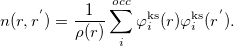
where $n_{\alpha }$ and $n_{\beta }$ are the number of alpha and beta electron respectively and, $\psi _ i$ are the Kohn-Sham orbitals. Thus, the total electron density is

$\begin{equation} \label{eq430} \rho (\ensuremath{\mathbf{r}}) =\rho _\alpha (\ensuremath{\mathbf{r}}) + \rho _\beta (\ensuremath{\mathbf{r}}) \end{equation}$

(4.32)

Within a finite basis set [28], the density is represented by

$\begin{equation} \label{eq431} \rho (\ensuremath{\mathbf{r}}) = \sum _{\mu \nu } {P_{\mu \nu }^{\mathrm{T}} \phi _\mu (\ensuremath{\mathbf{r}}) \phi _\nu (\ensuremath{\mathbf{r}})} \end{equation}$

(4.33)

The components of Eq. (4.28) can now be written as

$\displaystyle \label{eq432} E_{\mathrm{T}}^{}$	$\displaystyle =$	$\displaystyle \sum _{i=1}^{n_\alpha } \left\langle \psi _ i^\alpha \left\|-\frac{1}{2}\nabla ^2\right\|\psi _ i^{\alpha } \right\rangle + \sum _{i=1}^{n_\beta } \left\langle \psi _ i^\beta \left\|-\frac{1}{2}\nabla ^2\right\|\psi _ i^{\beta } \right\rangle \nonumber$
$\displaystyle$	$\displaystyle =$	$\displaystyle \sum _{\mu \nu } {P_{\mu \nu }^{\mathrm{T}} \left\langle \phi _\mu (\ensuremath{\mathbf{r}}) \left\|-\frac{1}{2}\nabla ^2\right\| \phi _\nu (\ensuremath{\mathbf{r}}) \right\rangle }$	(4.34)
$\displaystyle E_{\mathrm{V}}^{}$	$\displaystyle =$	$\displaystyle -\sum _{A=1}^ M Z_ A \frac{\rho (\ensuremath{\mathbf{r}})}{\|\ensuremath{\mathbf{r}}-\ensuremath{\mathbf{R}}_ A\|} d\ensuremath{\mathbf{r}} \nonumber$
$\displaystyle$	$\displaystyle =$	$\displaystyle -\sum _{\mu \nu } P_{\mu \nu }^{\mathrm{T}} \sum _ A \left\langle \phi _\mu (\ensuremath{\mathbf{r}}) \left\| \frac{Z_ A}{\|\ensuremath{\mathbf{r}}-\ensuremath{\mathbf{R}}_ A\|} \right\| \phi _\nu (\ensuremath{\mathbf{r}}) \right\rangle$	(4.35)
$\displaystyle E_{\mathrm{J}}^{}$	$\displaystyle =$	$\displaystyle \frac{1}{2}\left\langle \rho (\ensuremath{\mathbf{r}}_1) \left\| \frac{1}{\|\ensuremath{\mathbf{r}}_1 - \ensuremath{\mathbf{r}}_2\|} \right\| \rho (\ensuremath{\mathbf{r}}_2) \right\rangle \nonumber$
$\displaystyle$	$\displaystyle =$	$\displaystyle \frac{1}{2}\sum _{\mu \nu } \sum _{\lambda \sigma } P_{\mu \nu }^{\mathrm{T}} P_{\lambda \sigma }^{\mathrm{T}} \left(\mu \nu \vert \lambda \sigma \right)$	(4.36)
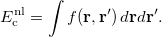
$\displaystyle E_{\mathrm{XC}}^{}$	$\displaystyle =$	$\displaystyle \int f\left[\rho (\ensuremath{\mathbf{r}}),\nabla \rho (\ensuremath{\mathbf{r}}),\ldots \right] d\ensuremath{\mathbf{r}} \label{E_ XC}$	(4.37)

Minimizing $E$ with respect to the unknown Kohn-Sham orbital coefficients yields a set of matrix equations exactly analogous to the UHF case

	$\displaystyle \label{eq436} \ensuremath{\mathbf{F}}^\alpha \ensuremath{\mathbf{C}}^\alpha = \varepsilon ^\alpha \ensuremath{\mathbf{SC}}^\alpha$		(4.38)
	$\displaystyle \ensuremath{\mathbf{F}}^\beta \ensuremath{\mathbf{C}}^\beta = \varepsilon ^\beta \ensuremath{\mathbf{SC}}^\beta$		(4.39)

where the Fock matrix elements are generalized to

	$\displaystyle \label{eq437} F_{\mu \nu }^\alpha = H_{\mu \nu }^{\mathrm{core}} + J_{\mu \nu } - F_{\mu \nu }^{\mathrm{XC}\alpha }$		(4.40)
	$\displaystyle F_{\mu \nu }^\beta = H_{\mu \nu }^{\mathrm{core}} + J_{\mu \nu } - F_{\mu \nu }^{\mathrm{XC}\beta }$		(4.41)

where $F_{\mu \nu }^{\mathrm{XC}\alpha }$ and $F_{\mu \nu }^{\mathrm{XC}\beta }$ are the exchange-correlation parts of the Fock matrices dependent on the exchange-correlation functional used. The Pople-Nesbet equations are obtained simply by allowing

$\begin{equation} \label{eq438} F_{\mu \nu }^{\mathrm{XC}\alpha } = K_{\mu \nu }^\alpha \end{equation}$

(4.42)

and similarly for the beta equation. Thus, the density and energy are obtained in a manner analogous to that for the Hartree-Fock method. Initial guesses are made for the MO coefficients and an iterative process applied until self consistency is obtained.

4.3.3 Exchange-Correlation Functionals

There are an increasing number of exchange and correlation functionals and hybrid DFT methods available to the quantum chemist, many of which are very effective. In short, there are nowadays five basic working types of functionals (five rungs on the Perdew’s “Jacob‘s Ladder"): those based on the local spin density approximation (LSDA) are on the first rung, those based on generalized gradient approximations (GGA) are on the second rung. Functionals that include not only density gradient corrections (as in the GGA functionals), but also a dependence on the electron kinetic energy density and/or the Laplacian of the electron density, occupy the third rung of the Jacob‘s Ladder and are known as “meta-GGA" functionals. The latter lead to a systematic, and often substantial improvement over GGA for thermochemistry and reaction kinetics. Among the meta-GGA functionals, a particular attention deserve the VSXC functional [29], the functional of Becke and Roussel for exchange [30], and for correlation [31] (the BR89B94 meta-GGA combination [31]). The latter functional did not receive enough popularity until recently, mainly because it was not representable in an analytic form. In Q-Chem, BR89B94 is implemented now self-consistently in a fully analytic form, based on the recent work [32]. The one and only non-empirical meta-GGA functional, the TPSS functional [33], was also implemented recently in Q-Chem [34]. Each of the above mentioned “pure” functionals can be combined with a fraction of exact (Hartree-Fock) non-local exchange energy replacing a similar fraction from the DFT local exchange energy. When a nonzero amount of Hartree-Fock exchange is used (less than a 100%), the corresponding functional is a hybrid extension (a global hybrid) of the parent “pure” functional. In most cases a hybrid functional would have one or more (up to 21 so far) linear mixing parameters that are fitted to experimental data. An exception is the hybrid extension of the TPSS meta-GGA functional, the non-empirical TPSSh scheme, which is also implemented now in Q-Chem [34].

The forth rung of functionals (“hyper-GGA” functionals) involve occupied Kohn-Sham orbitals as additional non-local variables [35, 36, 37, 38]. This helps tremendously in describing cases of strong inhomogeneity and strong non-dynamic correlation, that are evasive for global hybrids at GGA and meta-GGA levels of the theory. The success is mainly due to one novel feature of these functionals: they incorporate a 100% of exact (or HF) exchange combined with a hyper-GGA model correlation. Employing a 100% of exact exchange has been a long standing dream in DFT, but most previous attempts were unsuccessful. The correlation models used in the hyper-GGA schemes B05 [35] and PSTS [38], properly compensate the spuriously high non-locality of the exact exchange hole, so that cases of strong non-dynamic correlation become treatable.

In addition to some GGA and meta-GGA variables, the B05 scheme employs a new functional variable, namely, the exact-exchange energy density:

$\begin{equation} \label{HF_ X_ density} e^{{\mathrm{HF}}}_{X}(r) = -\frac{1}{2} \int dr^{'}\frac{|n(r,r^{'})|^{2}}{|r-r^{'}|} , \end{equation}$

(4.43)

where

$\begin{equation} \label{X-hole2} n(r,r^{'}) = \frac{1}{\rho (r)} \sum _{i}^{occ}\varphi _{i}^{\mathrm{ks}}(r) \varphi _{i}^{\mathrm{ks}}(r^{'}) . \end{equation}$

(4.44)

This new variable enters the correlation energy component in a rather sophisticated nonlinear manner [35]: This presents a huge challenge for the practical implementation of such functionals, since they require a Hartree-Fock type of calculation at each grid point, which renders the task impractical. Significant progress in implementing efficiently the B05 functional was reported only recently [39, 40]. This new implementation achieves a speed-up of the B05 calculations by a factor of 100 based on resolution-of-identity (RI) technique (the RI-B05 scheme) and analytical interpolations. Using this methodology, the PSTS hyper-GGA was also implemented in Q-Chem more recently [34]. For the time being only single-point SCF calculations are available for RI-B05 and RI-PSTS (the energy gradient will be available soon).

In contrast to B05 and PSTS, the forth-rung functional MCY employs a 100% global exact exchange, not only as a separate energy component of the functional, but also as a non-linear variable used the MCY correlation energy expression [36, 37]. Since this variable is the same at each grid point, it has to be calculated only once per SCF iteration. The form of the MCY correlation functional is deduced from known adiabatic connection and coordinate scaling relationships which, together with a few fitting parameters, provides a good correlation match to the exact exchange. The MCY functional [36] in its MCY2 version [37] is now implemented in Q-Chem, as described in Ref. [34].

The fifth-rung functionals include not only occupied Kohn-Sham orbitals, but also unoccupied orbitals, which improves further the quality of the exchange-correlation energy. The practical application so far of these consists of adding empirically a small fraction of correlation energy obtained from MP2-like post-SCF calculation [41, 42]. Such functionals are known as “double-hybrids”. A more detailed description of some these as implemented in Q-Chem is given in Sections 4.3.9 and 4.3.4.3. Finally, the so-called range-separated (or long-range corrected, LRC) functionals that employ exact exchange for the long-range part of the functional are showing excellent performance and considerable promise (see Section 4.3.4). In addition, many of the functionals can be augmented by an empirical dispersion correction, “-D” (see Section 4.3.6).

In summary, Q-Chem includes the following exchange and correlation functionals:

LSDA functionals:

Slater-Dirac (Exchange) [27]
Vokso-Wilk-Nusair (Correlation) [43]
Perdew-Zunger (Correlation) [44]
Wigner (Correlation) [45]
Perdew-Wang 92 (Correlation) [46]
Proynov-Kong 2009 (Correlation) [47]

GGA functionals:

Becke86 (Exchange) [48]
Becke88 (Exchange) [49]
PW86 (Exchange) [50]
refit PW86 (Exchange) [51]
Gill96 (Exchange) [52]
Gilbert-Gill99 (Exchange) [53]
Lee-Yang-Parr (Correlation) [54]
Perdew86 (Correlation) [55]
GGA91 (Exchange and correlation) [56]
mPW1PW91 (Exchange and Correlation) [57]
mPW1PBE (Exchange and Correlation)
mPW1LYP (Exchange and Correlation)
PBE (Exchange and correlation) [58, 59]
revPBE (Exchange) [60]
LB94 scheme (Exchange) [61]
LFA schemes (Exchange) [62]
AK13 (Exchange) [63]
PBE0 (25% Hartree-Fock exchange + 75% PBE exchange + 100% PBE correlation) [64]
PBE50 (50% Hartree-Fock exchange + 50% PBE exchange + 100% PBE correlation)
B3LYP (Exchange and correlation within a hybrid scheme) [65]
B3PW91 (B3 Exchange + PW91 correlation)
B3P86 (B3 Exchange + PW86 correlation)
B5050LYP (50% Hartree-Fock exchange + 5% Slater exchange + 42% Becke exchange + 100% LYP correlation) [66]
BHHLYP (50% Hartree-Fock exchange + 50% Becke exchange + 100% LYP correlation) [65]
O3LYP (Exchange and correlation) [67]
X3LYP (Exchange and correlation) [68]
CAM-B3LYP (Range separated exchange and LYP correlation) [69]
Becke97 (Exchange and correlation within a hybrid scheme) [70, 59]
Becke97-1 (Exchange and correlation within a hybrid scheme) [71, 59]
Becke97-2 (Exchange and correlation within a hybrid scheme) [72, 59]
B97-D (Exchange and correlation and empirical dispersion correction) [73]
HCTH (Exchange- correlation within a hybrid scheme) [71, 59]
HCTH-120 (Exchange- correlation within a hybrid scheme) [74, 59]
HCTH-147 (Exchange- correlation within a hybrid scheme) [74, 59]
HCTH-407 (Exchange- correlation within a hybrid scheme) [75, 59]
The $\omega$ B97X functionals developed by Chai and Head-Gordon [76] (Exchange and correlation within a hybrid scheme, with long-range correction, see further in this manual for details)
The $\omega$ B97X-D3 functional (Exchange-Correlation within a hybrid scheme, with long-range correction and dispersion correction, see futher in this manual for details) [77]
BNL (Exchange GGA functional) [78, 79]
BOP (Becke88 exchange plus the “one-parameter progressive” correlation functional, OP) [80]
PBEOP (PBE Exchange plus the OP correlation functional) [80]
SOGGA (Exchange plus the PBE correlation functional) [81]
SOGGA11 (Exchange and Correlation) [82]
SOGGA11-X (Exchange and Correlation within a hybrid scheme, with re-optimized SOGGA11 parameters) [83]
LRC- $\omega$ PBEPBE (Long-range corrected PBE exchange and PBE correlation) [84]
LRC- $\omega$ PBEhPBE (Long-range corrected hybrid PBE exchange and PBE correlation) [85]

Note: The OP correlation functional used in BOP has been parameterized for use with Becke88 exchange, whereas in the PBEOP functional, the same correlation ansatz is re-parameterized for use with PBE exchange. These two versions of OP correlation are available as the correlation functionals (B88)OP and (PBE)OP. The BOP functional, for example, consists of (B88)OP correlation combined with Becke88 exchange.

Meta-GGA functionals involving the kinetic energy density ( $\tau$ ), and or the Laplacian of the electron density:

VSXC (Exchange and Correlation) [29]
TPSS (Exchange and Correlation in a single non-empirical scheme) [33, 34]
TPSSh (Exchange and Correlation within a non-empirical hybrid scheme) [86]
BMK (Exchange and Correlation within a hybrid scheme) [87]
M05 (Exchange and Correlation within a hybrid scheme) [88, 89]
M05-2X (Exchange and Correlation within a hybrid scheme) [90, 89]
M06-L (Exchange and Correlation) [91, 89]
M06-HF (Exchange and Correlation within a hybrid scheme) [92, 89]
M06 (Exchange and Correlation within a hybrid scheme) [93, 89]
M06-2X (Exchange and Correlation within a hybrid scheme) [93, 89]
M08-HX (Exchange and Correlation within a hybrid scheme) [94]
M08-SO (Exchange and Correlation within a hybrid scheme) [94]
M11-L (Exchange and Correlation) [95]
M11 (Exchange and Correlation within a hybrid scheme, with long-range correction) [96]
BR89 (Exchange) [30, 32]
B94 (Correlation) [31, 32]
B95 (Correlation) [97]
B1B95 (Exchange and Correlation) [97]
PK06 (Correlation) [98]
The $\omega$ M05-D and $\omega$ M06-D3 functionals (Exchange-Correlation within a hybrid scheme, with long-range correction and dispersion correction, see futher in this manual for details) [99, 77]

Hyper-GGA functionals:

B05 (A full exact-exchange Kohn-Sham scheme of Becke that accounts for static correlation via real-space corrections) [35, 39, 40]
mB05 (Modified B05 method that has simpler functional form and SCF potential) [100]
PSTS (Hyper-GGA functional of Perdew-Staroverov-Tao-Scuseria) [38]
MCY2 (The adiabatic connection-based MCY2 functional) [36, 37, 34]
Fifth-rung, double-hybrid (DH) functionals:
$\omega$ B97X-2 (Exchange and Correlation within a DH generalization of the LC corrected $\omega$ B97X scheme) [42]
B2PLYP (another DH scheme proposed by Grimme, based on GGA exchange and correlation functionals) [73]
XYG3 and XYGJ-OS (an efficient DH scheme based on generalization of B3LYP) [101]
PBE0-DH [102] and PBE0-2 [103] functionals (non-empirical DH scheme based on the PBE functional).

In addition to the above functional types, Q-Chem contains the Empirical Density Functional 1 (EDF1), developed by Adamson, Gill and Pople [104]. EDF1 is a combined exchange and correlation functional that is specifically adapted to yield good results with the relatively modest-sized 6-31+G* basis set, by direct fitting to thermochemical data. It has the interesting feature that exact exchange mixing was not found to be helpful with a basis set of this size. Furthermore, for this basis set, the performance substantially exceeded the popular B3LYP functional, while the cost of the calculations is considerably lower because there is no need to evaluate exact (non-local) exchange. We recommend consideration of EDF1 instead of either B3LYP or BLYP for density functional calculations on large molecules, for which basis sets larger than 6-31+G* may be too computationally demanding.

EDF2, another Empirical Density Functional, was developed by Ching Yeh Lin and Peter Gill [105] in a similar vein to EDF1, but is specially designed for harmonic frequency calculations. It was optimized using the cc-pVTZ basis set by fitting into experimental harmonic frequencies and is designed to describe the potential energy curvature well. Fortuitously, it also performs better than B3LYP for thermochemical properties.

A few more words deserve the hybrid functionals [65], where several different exchange and correlation functionals can be combined linearly to form a hybrid functional. These have proven successful in a number of reported applications. However, since the hybrid functionals contain HF exchange they are more expensive that pure DFT functionals. Q-Chem has incorporated two of the most popular hybrid functionals, B3LYP [106] and B3PW91 [30], with the additional option for users to define their own hybrid functionals via the $xc_functional keyword (see user-defined functionals in Section 4.3.19, below). Among the latter, a recent new hybrid combination available in Q-Chem is the ’B3tLap’ functional, based on Becke’s B88 GGA exchange and the ’tLap’ (or ’PK06’) meta-GGA correlation [98, 107]. This hybrid combination is on average more accurate than B3LYP, BMK, and M06 functionals for thermochemistry and better than B3LYP for reaction barriers, while involving only five fitting parameters. Another hybrid functional in Q-Chem that deserves attention is the hybrid extension of the BR89B94 meta-GGA functional [31, 107]. This hybrid functional yields a very good thermochemistry results, yet has only three fitting parameters.

In addition, Q-Chem now includes the M05 and M06 suites of density functionals. These are designed to be used only with certain definite percentages of Hartree-Fock exchange. In particular, M06-L [91] is designed to be used with no Hartree-Fock exchange (which reduces the cost for large molecules), and M05 [88], M05-2X [90], M06, and M06-2X [93] are designed to be used with 28%, 56%, 27%, and 54% Hartree-Fock exchange. M06-HF [92] is designed to be used with 100% Hartree-Fock exchange, but it still contains some local DFT exchange because the 100% non-local Hartree-Fock exchange replaces only some of the local exchange.

Note: The hybrid functionals are not simply a pairing of an exchange and correlation functional, but are a combined exchange-correlation functional (i.e., B-LYP and B3LYP vary in the correlation contribution in addition to the exchange part).

4.3.4 Long-Range-Corrected DFT

As pointed out in Ref. Dreuw:2003 and elsewhere, the description of charge-transfer excited states within density functional theory (or more precisely, time-dependent DFT, which is discussed in Section 6.3) requires full (100%) non-local Hartree-Fock exchange, at least in the limit of large donor–acceptor distance. Hybrid functionals such as B3LYP [106] and PBE0 [64] that are well-established and in widespread use, however, employ only 20% and 25% Hartree-Fock exchange, respectively. While these functionals provide excellent results for many ground-state properties, they cannot correctly describe the distance dependence of charge-transfer excitation energies, which are enormously underestimated by most common density functionals. This is a serious problem in any case, but it is a catastrophic problem in large molecules and in clusters, where TDDFT often predicts a near-continuum of of spurious, low-lying charge transfer states [109, 110]. The problems with TDDFT’s description of charge transfer are not limited to large donor–acceptor distances, but have been observed at $\sim$ 2 separation, in systems as small as uracil– $(\rm H_2O)_4$ [109]. Rydberg excitation energies also tend to be substantially underestimated by standard TDDFT.

One possible avenue by which to correct such problems is to parameterize functionals that contain 100% Hartree-Fock exchange. To date, few such functionals exist, and those that do (such as M06-HF) contain a very large number of empirical adjustable parameters. An alternative option is to attempt to preserve the form of common GGAs and hybrid functionals at short range (i.e., keep the 25% Hartree-Fock exchange in PBE0) while incorporating 100% Hartree-Fock exchange at long range. Functionals along these lines are known variously as “Coulomb-attenuated” functionals, “range-separated” functionals, or (our preferred designation) “long-range-corrected” (LRC) density functionals. Whatever the nomenclature, these functionals are all based upon a partition of the electron-electron Coulomb potential into long- and short-range components, using the error function (erf):

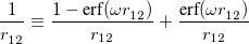$\begin{equation} \label{eq:erf_ partition} \frac{1}{r_{12}^{}} \equiv \frac{1-\mbox{erf}(\omega r_{12}^{})}{r_{12}} + \frac{\mbox{erf}(\omega r_{12}^{})}{r_{12}} \; \end{equation}$

(4.45)

The first term on the right in Eq. () is singular but short-range, and decays to zero on a length scale of $\sim 1/\omega$ , while the second term constitutes a non-singular, long-range background. The basic idea of LRC-DFT is to utilize the short-range component of the Coulomb operator in conjunction with standard DFT exchange (including any component of Hartree-Fock exchange, if the functional is a hybrid), while at the same time incorporating full Hartree-Fock exchange using the long-range part of the Coulomb operator. This provides a rigorously correct description of the long-range distance dependence of charge-transfer excitation energies, but aims to avoid contaminating short-range exchange-correlation effects with extra Hartree-Fock exchange.

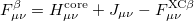
Consider an exchange-correlation functional of the form

$\begin{equation} \label{eq:Exc_ standard} E_{\rm XC}^{} = E_{\rm C}^{} + E_{\rm X}^{\rm GGA} + C_{\rm HF}^{} \, E_{\rm X}^{\rm HF} \end{equation}$

(4.46)

in which $E_{\rm C}^{}$ is the correlation energy, $E_{\rm X}^{\rm GGA}$ is the (local) GGA exchange energy, and $E_{\rm X}^{\rm HF}$ is the (non-local) Hartree-Fock exchange energy. The constant $C_{\rm HF}^{}$ denotes the fraction of Hartree-Fock exchange in the functional, therefore $C_{\rm HF}^{} = 0$ for GGAs, $C_{\rm HF}^{} = 0.20$ for B3LYP, $C_{\rm HF}^{} = 0.25$ for PBE0, etc.. The LRC version of the generic functional in Eq. () is

$\begin{equation} \label{eq:Exc_ LRC} E_{\rm XC}^{\rm LRC} = E_{\rm C}^{} + E_{\rm X}^{\rm GGA, SR} + C_{\rm HF}^{}\, E_{\rm X}^{\rm HF, SR} + E_{\rm X}^{\rm HF, LR} \end{equation}$

(4.47)

in which the designations “SR” and “LR” in the various exchange energies indicate that these components of the functional are evaluated using either the short-range (SR) or the long-range (LR) component of the Coulomb operator. (The correlation energy $E_{\rm C}^{}$ is evaluated using the full Coulomb operator.) The LRC functional in Eq. () incorporates full Hartree-Fock exchange in the asymptotic limit via the final term, $E_{\rm X}^{\rm HF, LR}$ . To fully specify the LRC functional, one must choose a value for the range separation parameter $\omega$ in Eq. (); in the limit $\omega \rightarrow 0$ , the LRC functional in Eq. () reduces to the original functional in Eq. (), while the $\omega \rightarrow \infty$ limit corresponds to a new functional, $E_{\rm XC}^{} = E_{\rm C}^{} + E_{\rm X}^{\rm HF}$ . It is well known that full Hartree-Fock exchange is inappropriate for use with most contemporary GGA correlation functionals, so the latter limit is expected to perform quite poorly. Values of $\omega > 1.0~ \mbox{bohr}^{-1}$ are probably not worth considering [111, 84].

Evaluation of the short- and long-range Hartree-Fock exchange energies is straightforward [112], so the crux of LRC-DFT rests upon the form of the short-range GGA exchange energy. Several different short-range GGA exchange functionals are available in Q-Chem, including short-range variants of B88 and PBE exchange described by Hirao and co-workers [113, 114], an alternative formulation of short-range PBE exchange proposed by Scuseria and co-workers [115], and several short-range variants of B97 introduced by Chai and Head-Gordon [76, 116, 117, 42]. The reader is referred to these papers for additional methodological details.

These LRC-DFT functionals have been shown to remove the near-continuum of spurious charge-transfer excited states that appear in large-scale TDDFT calculations [111]. However, certain results depend sensitively upon the range-separation parameter $\omega$ [110, 111, 84, 85], and the results of LRC-DFT calculations must therefore be interpreted with caution, and probably for a range of $\omega$ values. In two recent benchmark studies of several LRC density functionals, Rohrdanz and Herbert [84, 85] have considered the errors engendered, as a function of $\omega$ , in both ground-state properties and also TDDFT vertical excitation energies. In Ref. Lange:2008, the sensitivity of valence excitations versus charge-transfer excitation energies in TDDFT was considered, again as a function of $\omega$ . A careful reading of these references is suggested prior to performing any LRC-DFT calculations.

Within Q-Chem 3.2, there are three ways to perform LRC-DFT calculations.

4.3.4.1 LRC-DFT with the $\bm@general \boldmath \m@ne \mv@bold \bm@command {\mu }$ B88, $\bm@general \boldmath \m@ne \mv@bold \bm@command {\mu }$ PBE, and $\bm@general \boldmath \m@ne \mv@bold \bm@command {\omega }$ PBE exchange functionals

The form of $E_{\rm X}^{\rm GGA, SR}$ is different for each different GGA exchange functional, and short-range versions of B88 and PBE exchange are available in Q-Chem through the efforts of the Herbert group. Versions of B88 and PBE, in which the Coulomb attenuation is performed according to the procedure of Hirao [114], are denoted as $\mu$ B88 and $\mu$ PBE, respectively (since $\mu$ , rather than $\omega$ , is the Hirao group’s notation for the range-separation parameter). Alternatively, a short-range version of PBE exchange called $\omega$ PBE is available, which is constructed according to the prescription of Scuseria and co-workers [115].

These short-range exchange functionals can be used in the absence of long-range Hartree-Fock exchange, and using a combination of $\omega$ PBE exchange and PBE correlation, a user could, for example, employ the short-range hybrid functional recently described by Heyd, Scuseria, and Ernzerhof [118]. Short-range hybrids appear to be most appropriate for extended systems, however. Thus, within Q-Chem, short-range GGAs should be used with long-range Hartree-Fock exchange, as in Eq. . Long-range Hartree-Fock exchange is requested by setting LRC_DFT to TRUE.

LRC-DFT is thus available for any functional whose exchange component consists of some combination of Hartree-Fock, B88, and PBE exchange (e.g., BLYP, PBE, PBE0, BOP, PBEOP, and various user-specified combinations, but not B3LYP or other functionals whose exchange components are more involved). Having specified such a functional via the EXCHANGE and CORRELATION variables, a user may request the corresponding LRC functional by setting LRC_DFT to TRUE. Long-range-corrected variants of PBE0, BOP, and PBEOP must be obtained through the appropriate user-specified combination of exchange and correlation functionals (as demonstrated in the example below). In any case, the value of $\omega$ must also be specified by the user. Analytic energy gradients are available but analytic Hessians are not. TDDFT vertical excitation energies are also available.

LRC_DFT

Controls the application of long-range-corrected DFT

TYPE:

LOGICAL

DEFAULT:

FALSE

OPTIONS:

FALSE

(or 0) Do not apply long-range correction.

TRUE

(or 1) Use the long-range-corrected version of the requested functional.

RECOMMENDATION:

Long-range correction is available for any combination of Hartree-Fock, B88, and PBE exchange (along with any stand-alone correlation functional).

OMEGA

Sets the Coulomb attenuation parameter $\omega$ .

TYPE:

INTEGER

DEFAULT:

No default

OPTIONS:

$n$

Corresponding to $\omega = n/1000$ , in units of bohr $^{-1}$

RECOMMENDATION:

None

Example 4.23 Application of LRC- $\mu$ BOP to $\rm (H_2O)_2^-$ .

$comment
   To obtain LRC-BOP, a short-range version of BOP must be specified,    
   using muB88 short-range exchange plus (B88)OP correlation, which is 
   the version of OP parameterized for use with B88.
$end

$molecule
-1 2
O           1.347338    -.017773    -.071860
H           1.824285     .813088     .117645
H           1.805176    -.695567     .461913
O          -1.523051    -.002159    -.090765
H           -.544777    -.024370    -.165445
H          -1.682218     .174228     .849364
$end

$rem
   EXCHANGE      GEN    
   BASIS         6-31(1+,3+)G*
   LRC_DFT       TRUE
   OMEGA         330      ! = 0.330 a.u.
$end

$xc_functional
   C    (B88)OP    1.0
   X    muB88      1.0
$end

Regarding the choice of functionals and $\omega$ values, it has been found that the Hirao and Scuseria ansatz afford virtually identical TDDFT excitation energies, for all values of $\omega$ [85]. Thus, functionals based on $\mu$ PBE versus $\omega$ PBE provide the same excitation energies, as a function of $\omega$ . However, the $\omega$ PBE functional appears to be somewhat superior in the sense that it can provide accurate TDDFT excitation energies and accurate ground-state properties using the same value of $\omega$ [85], whereas this does not seem to be the case for functionals based on $\mu$ B88 or $\mu$ PBE [84].

Recently, Rohrdanz et al. [85] have published a thorough benchmark study of both ground- and excited-state properties, using the “LRC- $\omega$ PBEh” functional, a hybrid (hence the “h”) that contains a fraction of short-range Hartree-Fock exchange in addition to full long-range Hartree-Fock exchange:

$\begin{equation} \label{eq:LRC-wPBEh} E_{\rm XC}^{}(\mbox{LRC-}\omega \mbox{PBEh}) = E_{\rm C}^{}(\mbox{PBE}) + E_{\rm X}^{\rm SR}(\omega \mbox{PBE}) + C_{\rm HF}^{}\, E_{\rm X}^{\rm SR}(\mbox{HF}) + E_{\rm X}^{\rm LR}(\mbox{HF}) \end{equation}$

(4.48)

The statistically-optimal parameter set, consider both ground-state properties and TDDFT excitation energies together, was found to be $C_{\rm HF}^{} = 0.2$ and $\omega = 0.2$ bohr $^{-1}$ [85]. With these parameters, the LRC- $\omega$ PBEh functional outperforms the traditional hybrid functional PBE0 for ground-state atomization energies and barrier heights. For TDDFT excitation energies corresponding to localized excitations, TD-PBE0 and TD-LRC- $\omega$ PBEh show similar statistical errors of $\sim$ 0.3 eV, but the latter functional also exhibits only $\sim$ 0.3 eV errors for charge-transfer excitation energies, whereas the statistical error for TD-PBE0 charge-transfer excitation energies is 3.0 eV! Caution is definitely warranted in the case of charge-transfer excited states, however, as these excitation energies are very sensitive to the precise value of $\omega$ [110, 85]. It was later found that the parameter set ( $C_{\rm HF}^{} = 0$ , $\omega = 0.3$ bohr $^{-1}$ ) provides similar (statistical) performance to that described above, although the predictions for specific charge-transfer excited states can be somewhat different as compared to the original parameter set [110].

Example 4.24 Application of LRC- $\omega$ PBEh to the $\rm C_2H_4$ — $\rm C_2F_4$ hetero-dimer at 5 separation.

$comment
    This example uses the "optimal" parameter set discussed above.  
    It can also be run by setting "EXCHANGE LRC-WPBEhPBE".
$end

$molecule
0 1
C           0.670604    0.000000    0.000000
C          -0.670604    0.000000    0.000000
H           1.249222    0.929447    0.000000
H           1.249222   -0.929447    0.000000
H          -1.249222    0.929447    0.000000
H          -1.249222   -0.929447    0.000000
C           0.669726    0.000000    5.000000
C          -0.669726    0.000000    5.000000
F           1.401152    1.122634    5.000000
F           1.401152   -1.122634    5.000000
F          -1.401152   -1.122634    5.000000
F          -1.401152    1.122634    5.000000
$end

$rem
   EXCHANGE      GEN    
   BASIS         6-31+G*
   LRC_DFT       TRUE
   OMEGA         200      ! = 0.2 a.u.
   CIS_N_ROOTS   4
   CIS_TRIPLETS  FALSE
$end

$xc_functional
   C    PBE        1.00
   X    wPBE       0.80
   X    HF         0.20
$end

Both LRC functionals and asymptotic corrections (Section 4.3.10.1) are thought to reduce self-interaction error in approximate density functional theory. A convenient way to quantify (or at least depict) this error is by plotting the DFT energy as a function of the (fractional) number of electrons, $N$ , as the exchange-correlation potential changes discontinuously as $N$ passes through an integer, and thus a plot of $E$ versus $N$ abruptly changes slope at integer values of $N$ [119]. Examination of such plots has been suggested as a means to “tune” the fraction of short-range exchange in an LRC function [120], while the range separation parameter can be tuned so as to achieve the condition (exact for the Hohenberg-Kohn functional) $\epsilon _{\rm HOMO}^{} = -\mbox{IE}$ , where IE denotes the molecule’s lowest ionization energy [121].

Example 4.25 Example of a DFT job with a fraction number of electrons. Here, we make the $-1.x$ anion of fluoride by subracting a fraction of an electron from the HOMO of F $^{2-}$ .

$comment
    Subtracting a whole electron recovers the energy of F-.
    Adding electrons to the LUMO is possible as well.
$end

$rem
exchangeh           b3lyp
basis               6-31+G*
fractional_electron -500  ! /divide by 1000 to get the fraction, -0.5 here.
$end

$molecule
-2 2
F
$end

4.3.4.2 LRC-DFT with the BNL Functional

The Baer-Neuhauser-Livshits (BNL) functional [78, 79] is also based on the range separation of the Coulomb operator in Eq. . Its functional form resembles Eq. :

$\begin{equation} \label{eq:Exc_ LRC2} E_{\rm XC}^{} = E_{\rm C}^{} + C_{\rm GGA,X} E_{\rm X}^{\rm GGA, SR} + E_{\rm X}^{\rm HF, LR} \end{equation}$

(4.49)

where the recommended GGA correlation functional is LYP. The recommended GGA exchange functional is BNL, which is described by a local functional [122]. For ground state properties, the optimized value for $C_{GGA,X}$ (scaling factor for the BNL exchange functional) was found to be 0.9.

The value of $\omega$ in BNL calculations can be chosen in several different ways. For example, one can use the optimized value $\omega$ =0.5 bohr $^{-1}$ . For calculation of excited states and properties related to orbital energies, it is strongly recommend to tune $\omega$ as described below[121, 123].

System-specific optimization of $\omega$ is based on Koopmans conditions that would be satisfied for the exact functional[121], that is, $\omega$ is varied until the Koopmans IE/EA for the HOMO/LUMO is equal to $\Delta E$ IE/EA. Based on published benchmarks [79, 124], this system-specific approach yields the most accurate values of IEs and excitation energies.

The script that optimizes $\omega$ is called OptOmegaIPEA.pl and is located in the $QC/bin directory. The script optimizes $\omega$ in the range 0.1-0.8 (100-800). See the script for the instructions how to modify the script to optimize in a broader range. To execute the script, you need to create three inputs for a BNL job using the same geometry and basis set for a neutral molecule (N.in), anion (M.in), and cation (P.in), and then type 'OptOmegaIPEA.pl >& optomega'. The script will run creating outputs for each step (N_*, P_*, M_*) writing the optimization output into optomega.

A similar script, OptOmegaIP.pl, will optimize $\omega$ to satisfy the Koopmans condition for the IP only. This script minimizes $J=(IP+\epsilon _{HOMO})^2$ , not the absolute values.

Note: (i) If the system does not have positive EA, then the tuning should be done according to the IP condition only. The IPEA script will yield a wrong value of $\omega$ in such cases.
(ii) In order for the scripts to work, one must specify SCF_FINAL_PRINT=1 in the inputs. The scripts look for specific regular expressions and will not work correctly without this keyword.
(iii) When tuning omega we recommend taking the amount of X BNL in the XC part as 1.0 and not 0.9.

The $xc_functional keyword for a BNL calculation reads:

$xc_functional
  X HF 1.0
  X BNL 0.9
  C LYP 1.0
$end

and the $rem keyword reads

$rem
  EXCHANGE      GENERAL
  SEPARATE_JK   TRUE
  OMEGA         500     != 0.5 Bohr$^{-1}$
  DERSCREEN     FALSE   !if performing unrestricted calcn
  IDERIV        0       !if performing unrestricted Hessian evaluation
$end

4.3.4.3 LRC-DFT with $\omega$ B97, $\omega$ B97X, $\omega$ B97X-D, and $\omega$ B97X-2 Functionals

Also available in Q-Chem are the $\omega$ B97 [76], $\omega$ B97X [76], $\omega$ B97X-D [116], and $\omega$ B97X-2 [42] functionals, recently developed by Chai and Head-Gordon. These authors have proposed a very simple ansatz to extend any E $_{\text {X}}^{\text {GGA}}$ to E $_{\text {X}}^{\text {GGA,SR}}$ , as long as the SR operator has considerable spatial extent [76, 117]. With the use of flexible GGAs, such as Becke97 functional [70], their new LRC hybrid functionals [76, 116, 117] outperform the corresponding global hybrid functionals (i.e., B97) and popular hybrid functionals (e.g., B3LYP) in thermochemistry, kinetics, and non-covalent interactions, which has not been easily achieved by the previous LRC hybrid functionals. In addition, the qualitative failures i of the commonly used hybrid density functionals in some “difficult problems”, such as dissociation of symmetric radical cations and long-range charge-transfer excitations, are significantly reduced by these new functionals [76, 116, 117]. Analytical gradients and analytical Hessians are available for $\omega$ B97, $\omega$ B97X, and $\omega$ B97X-D.

Example 4.26 Application of $\omega$ B97 functional to nitrogen dimer.

$comment
Geometry optimization, followed by a TDDFT calculation.
$end

$molecule
0 1
N1
N2 N1 1.1
$end

$rem
jobtype         opt
exchange        omegaB97
basis           6-31G*
$end

@@@

$molecule
READ
$end

$rem
jobtype         sp
exchange        omegaB97
basis           6-31G*
scf_guess       READ
cis_n_roots     10
rpa             true
$end

Example 4.27 Application of $\omega$ B97X functional to nitrogen dimer.

$comment
Frequency calculation (with analytical Hessian methods).
$end

$molecule
0 1
N1
N2 N1 1.1
$end

$rem
jobtype         freq
exchange        omegaB97X
basis           6-31G*
$end

Among these new LRC hybrid functionals, $\omega$ B97X-D is a DFT-D (density functional theory with empirical dispersion corrections) functional, where the total energy is computed as the sum of a DFT part and an empirical atomic-pairwise dispersion correction. Relative to $\omega$ B97 and $\omega$ B97X, $\omega$ B97X-D is significantly superior for non-bonded interactions, and very similar in performance for bonded interactions. However, it should be noted that the remaining short-range self-interaction error is somewhat larger for $\omega$ B97X-D than for $\omega$ B97X than for $\omega$ B97. A careful reading of Refs. Chai:2008a,Chai:2008b,Chai:2008c is suggested prior to performing any DFT and TDDFT calculations based on variations of $\omega$ B97 functional. $\omega$ B97X-D functional automatically involves two keywords for the dispersion correction, DFT_D and DFT_D_A, which are described in Section 4.3.6.

Example 4.28 Application of $\omega$ B97X-D functional to methane dimer.

$comment
Geometry optimization.
$end

$molecule
0 1
C       0.000000    -0.000323     1.755803
H      -0.887097     0.510784     1.390695
H       0.887097     0.510784     1.390695
H       0.000000    -1.024959     1.393014
H       0.000000     0.001084     2.842908
C       0.000000     0.000323    -1.755803
H       0.000000    -0.001084    -2.842908
H      -0.887097    -0.510784    -1.390695
H       0.887097    -0.510784    -1.390695
H       0.000000     1.024959    -1.393014
$end

$rem
jobtype         opt
exchange        omegaB97X-D
basis           6-31G*
$end

Similar to the existing double-hybrid density functional theory (DH-DFT) [41, 125, 126, 127, 101], which is described in Section 4.3.9, LRC-DFT can be extended to include non-local orbital correlation energy from second-order Møller-Plesset perturbation theory (MP2) [128], that includes a same-spin (ss) component $E_{c}^{ss}$ , and an opposite-spin (os) component $E_{c}^{os}$ of PT2 correlation energy. The two scaling parameters, $c_{ss}$ and $c_{os}$ , are introduced to avoid double-counting correlation with the LRC hybrid functional.

$\begin{equation} \label{eq:dft2} E_{\text {total}} = E_{\text {LRC-DFT}} + c_{ss} E_{c}^{ss} + c_{os} E_{c}^{os} \end{equation}$

(4.50)

Among the $\omega$ B97 series, $\omega$ B97X-2 [42] is a long-range corrected double-hybrid (DH) functional, which can greatly reduce the self-interaction errors (due to its high fraction of Hartree-Fock exchange), and has been shown significantly superior for systems with bonded and non-bonded interactions. Due to the sensitivity of PT2 correlation energy with respect to the choices of basis sets, $\omega$ B97X-2 was parameterized with two different basis sets. $\omega$ B97X-2(LP) was parameterized with the 6-311++G(3df,3pd) basis set (the large Pople type basis set), while $\omega$ B97X-2(TQZ) was parameterized with the TQ extrapolation to the basis set limit. A careful reading of Ref. Chai:2009 is thus highly advised.

$\omega$ B97X-2(LP) and $\omega$ B97X-2(TQZ) automatically involve three keywords for the PT2 correlation energy, DH, SSS_FACTOR and SOS_FACTOR, which are described in Section 4.3.9. The PT2 correlation energy can also be computed with the efficient resolution-of-identity (RI) methods (see Section 5.5).

Example 4.29 Application of $\omega$ B97X-2(LP) functional to LiH molecules.

$comment
Geometry optimization and frequency calculation on LiH, followed by
single-point calculations with non-RI and RI approaches.
$end

$molecule
0 1
H
Li H 1.6
$end

$rem
jobtype         opt
exchange        omegaB97X-2(LP)
correlation     mp2
basis           6-311++G(3df,3pd)
$end

@@@

$molecule
READ
$end

$rem
jobtype         freq
exchange        omegaB97X-2(LP)
correlation     mp2
basis           6-311++G(3df,3pd)
$end

@@@

$molecule
READ
$end

$rem
jobtype         sp
exchange        omegaB97X-2(LP)
correlation     mp2
basis           6-311++G(3df,3pd)
$end

@@@

$molecule
READ
$end

$rem
jobtype          sp
exchange         omegaB97X-2(LP)
correlation      rimp2
basis            6-311++G(3df,3pd)
aux_basis        rimp2-aug-cc-pvtz
$end

Example 4.30 Application of $\omega$ B97X-2(TQZ) functional to LiH molecules.

$comment
Single-point calculations on LiH.
$end

$molecule
0 1
H
Li H 1.6
$end

$rem
jobtype         sp
exchange        omegaB97X-2(TQZ)
correlation     mp2
basis           cc-pvqz
$end

@@@

$molecule
READ
$end

$rem
jobtype         sp
exchange        omegaB97X-2(TQZ)
correlation     rimp2
basis           cc-pvqz
aux_basis       rimp2-cc-pvqz
$end

4.3.4.4 LRC-DFT with $\omega$ M05-D, $\omega$ M06-D3 and $\omega$ B97X-D3 Functionals

$\omega$ M05-D [99], $\omega$ M06-D3 and $\omega$ B97X-D3 functionals [77], developed by the Chai group, improve on the $\omega$ B97X-D functional mentioned above. Similar to the $\omega$ B97X-D functional, these functionals also involves emperical atomic-pairwise dispersion corrections, and automatically involves the keywords for dispersion correction.

Analytical gradient is available for all three functionals in Q-Chem, and analytical Hessian is available for $\omega$ B97X-D3.

Example 4.31 Applications of $\omega$ M05-D to a methane dimer.

$comment
Geometry optimization, followed by single-point TDDFT calculations
using a larger basis set.
$end

$molecule
0 1
C       0.000000    -0.000323     1.755803
H      -0.887097     0.510784     1.390695
H       0.887097     0.510784     1.390695
H       0.000000    -1.024959     1.393014
H       0.000000     0.001084     2.842908
C       0.000000     0.000323    -1.755803
H       0.000000    -0.001084    -2.842908
H      -0.887097    -0.510784    -1.390695
H       0.887097    -0.510784    -1.390695
H       0.000000     1.024959    -1.393014
$end

$rem
jobtype         opt
method          wM05-D
basis           6-31G*
$end

@@@

$molecule
READ
$end

$rem
jobtype         sp
method          wM05-D
basis           6-311++G**
cis_n_roots     30
rpa             true
$end

Example 4.32 Applications of $\omega$ M06-D3 to a methane dimer.

$comment
Geometry optimization, followed by single-point TDDFT calculations
using a larger basis set.
$end

$molecule
0 1
C       0.000000    -0.000323     1.755803
H      -0.887097     0.510784     1.390695
H       0.887097     0.510784     1.390695
H       0.000000    -1.024959     1.393014
H       0.000000     0.001084     2.842908
C       0.000000     0.000323    -1.755803
H       0.000000    -0.001084    -2.842908
H      -0.887097    -0.510784    -1.390695
H       0.887097    -0.510784    -1.390695
H       0.000000     1.024959    -1.393014
$end

$rem
jobtype         opt
method          wM06-D3
basis           6-31G*
$end

@@@

$molecule
READ
$end

$rem
jobtype         sp
method          wM06-D3
basis           6-311++G**
cis_n_roots     30
rpa             true
$end

Example 4.33 Applications of $\omega$ B97X-D3 to a methane dimer.

$comment
Geometry optimization, followed by single-point TDDFT calculations
using a larger basis set (with analytical Hessian).
$end

$molecule
0 1
C       0.000000    -0.000323     1.755803
H      -0.887097     0.510784     1.390695
H       0.887097     0.510784     1.390695
H       0.000000    -1.024959     1.393014
H       0.000000     0.001084     2.842908
C       0.000000     0.000323    -1.755803
H       0.000000    -0.001084    -2.842908
H      -0.887097    -0.510784    -1.390695
H       0.887097    -0.510784    -1.390695
H       0.000000     1.024959    -1.393014
$end

$rem
jobtype         opt
method          wB97X-D3
basis           6-31G*
$end

@@@

$molecule
READ
$end

$rem
jobtype         sp
method          wB97X-D3
basis           6-311++G**
cis_n_roots     30
rpa             true
$end

4.3.4.5 LRC-DFT with the M11 Family of Functionals

The Minnesota family of functional by Truhlar’s group has been recently updated by adding two new functionals: M11-L [95] and M11 [96]. The M11 functional is a long-range corrected meta-GGA, obtained by using the LRC scheme of Chai and Head-Gordon (see above), with the successful parameterization of the Minnesota meta-GGA functionals:

$\begin{equation} E^{M11}_{xc} = \left( \frac{X}{100} \right) E^{SR-HF}_ x + \left( 1 - \frac{X}{100} \right) E^{SR-M11}_ x + E^{LR-HF}_ x + E^{M11}_ c \end{equation}$

(4.51)

with the percentage of Hartree-Fock exchange at short range X being 42.8. An extension of the LRC scheme to local functional (no HF exchange) was introduced in the M11-L functional by means of the dual-range exchange:

$\begin{equation} E^{M11-L}_{xc} = E^{SR-M11}_ x + E^{LR-M11}_ x + E^{M11-L}_ c \end{equation}$

(4.52)

The correct long-range scheme is selected automatically with the input keywords. A careful reading of the references [95, 96] is suggested prior to performing any calculations with the M11 functionals.

Example 4.34 Application of M11 functional to water molecule

$comment
Optimization of H2O with M11
$end

$molecule
0 1
O 0.000000 0.000000  0.000000
H 0.000000 0.000000  0.956914
H 0.926363 0.000000 -0.239868
$end

$rem
jobtype opt 
exchange m11 
basis 6-31+G(d,p)
$end

4.3.5 Nonlocal Correlation Functionals

Q-Chem includes four nonlocal correlation functionals that describe long-range dispersion (i.e. van der Waals) interactions:

vdW-DF-04, developed by Langreth, Lundqvist, and coworkers [129, 130] and implemented as described in Ref. [131];
vdW-DF-10 (also known as vdW-DF2), which is a re-parameterization [132] of vdW-DF-04, implemented in the same way as its precursor [131];
VV09, developed [133] and implemented [134] by Vydrov and Van Voorhis;
VV10 by Vydrov and Van Voorhis [135].

All these functionals are implemented self-consistently and analytic gradients with respect to nuclear displacements are available [131, 134, 135]. The nonlocal correlation is governed by the $rem variable NL_CORRELATION, which can be set to one of the four values: vdW-DF-04, vdW-DF-10, VV09, or VV10. Note that vdW-DF-04, vdW-DF-10, and VV09 functionals are used in combination with LSDA correlation, which must be specified explicitly. For instance, vdW-DF-10 is invoked by the following keyword combination:

CORRELATION        PW92
NL_CORRELATION     vdW-DF-10

VV10 is used in combination with PBE correlation, which must be added explicitly. In addition, the values of two parameters, $C$ and $b$ must be specified for VV10. These parameters are controlled by the $rem variables NL_VV_C and NL_VV_B, respectively. For instance, to invoke VV10 with $C = 0.0093$ and $b = 5.9$ , the following input is used:

CORRELATION        PBE
NL_CORRELATION     VV10
NL_VV_C            93
NL_VV_B            590

The variable NL_VV_C may also be specified for VV09, where it has the same meaning. By default, $C = 0.0089$ is used in VV09 (i.e. NL_VV_C is set to 89). However, in VV10 neither $C$ nor $b$ are assigned a default value and must always be provided in the input.

As opposed to local (LSDA) and semilocal (GGA and meta-GGA) functionals, evaluated as a single 3D integral over space [see Eq. ()], non-local functionals require double integration over the spatial variables:

$\begin{equation} E_{\rm c}^{\rm nl} = \int f(\ensuremath{\mathbf{r}},\ensuremath{\mathbf{r'}}) \, d\ensuremath{\mathbf{r}} d\ensuremath{\mathbf{r'}}. \end{equation}$

(4.53)

In practice, this double integration is performed numerically on a quadrature grid [131, 134, 135]. By default, the SG-1 quadrature (described in Section 4.3.15 below) is used to evaluate $E_{\rm c}^{\rm nl}$ , but a different grid can be requested via the $rem variable NL_GRID. The non-local energy is rather insensitive to the fineness of the grid, so that SG-1 or even SG-0 grids can be used in most cases. However, a finer grid may be required for the (semi)local parts of the functional, as controlled by the XC_GRID variable.

Example 4.35 Geometry optimization of the methane dimer using VV10 with rPW86 exchange.


$molecule
0 1
C   0.000000  -0.000140   1.859161
H  -0.888551   0.513060   1.494685
H   0.888551   0.513060   1.494685
H   0.000000  -1.026339   1.494868
H   0.000000   0.000089   2.948284
C   0.000000   0.000140  -1.859161
H   0.000000  -0.000089  -2.948284
H  -0.888551  -0.513060  -1.494685
H   0.888551  -0.513060  -1.494685
H   0.000000   1.026339  -1.494868
$end

$rem
JobType            Opt
BASIS              aug-cc-pVTZ
EXCHANGE           rPW86
CORRELATION        PBE
XC_GRID            75000302
NL_CORRELATION     VV10
NL_GRID            1
NL_VV_C            93
NL_VV_B            590
$end

In the above example, an EML-(75,302) grid is used to evaluate the rPW86 exchange and PBE correlation, but a coarser SG-1 grid is used for the non-local part of VV10.

4.3.6 DFT-D Methods

4.3.6.1 Empirical dispersion correction from Grimme

Thanks to the efforts of the Sherrill group, the popular empirical dispersion corrections due to Grimme [73] are now available in Q-Chem. Energies, analytic gradients, and analytic second derivatives are available. Grimme’s empirical dispersion corrections can be added to any of the density functionals available in Q-Chem.

DFT-D methods add an extra term,

$\displaystyle \label{eqn:C6} E_{\rm disp}$	$\displaystyle =$	$\displaystyle -s_6 \sum _ A \sum _{B<A} \frac{C_{6}^{AB}}{R_{AB}^{6}}f_{dmp}(R_{AB})$	(4.54)
$\displaystyle C_{6}^{AB}$	$\displaystyle =$	$\displaystyle \sqrt {C_{6}^{A}C_{6}^{B}},$	(4.55)
$\displaystyle f_{\rm dmp}(R_{AB})$	$\displaystyle =$	$\displaystyle \frac{1}{1+e^{-d(R_{AB}/R_{AB}^0 - 1)}}$	(4.56)

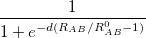
where $s_6$ is a global scaling parameter (near unity), $f_{\rm dmp}$ is a damping parameter meant to help avoid double-counting correlation effects at short range, $d$ is a global scaling parameter for the damping function, and $R_{AB}^0$ is the sum of the van der Waals radii of atoms A and B.

DFT-D using Grimme’s parameters may be turned on using

DFT_D     EMPIRICAL_GRIMME

Grimme has suggested scaling factors $s_6$ of 0.75 for PBE, 1.2 for BLYP, 1.05 for BP86, and 1.05 for B3LYP; these are the default values of $s_6$ when those functionals are used. Otherwise, the default value of $s_6$ is 1.0.

It is possible to specify different values of $s_6$ , $d$ , the atomic $C_6$ coefficients, or the van der Waals radii by using the $empirical_dispersion keyword; for example:

$empirical_dispersion
S6 1.1
D 10.0
C6 Ar 4.60 Ne 0.60
VDW_RADII Ar 1.60 Ne 1.20
$end

Any values not specified explicitly will default to the values in Grimme’s model.

4.3.6.2 Empirical dispersion correction from Chai and Head-Gordon

The empirical dispersion correction from Chai and Head-Gordon [116] employs a different damping function and can be activated by using

DFT_D     EMPIRICAL_CHG

It uses another keyword DFT_D_A to control the strength of dispersion corrections.

DFT_D

Controls the application of DFT-D or DFT-D3 scheme.

TYPE:

LOGICAL

DEFAULT:

None

OPTIONS:

FALSE

(or 0) Do not apply the DFT-D or DFT-D3 scheme

EMPIRICAL_GRIMME

dispersion correction from Grimme

EMPIRICAL_CHG

dispersion correction from Chai and Head-Gordon

EMPIRICAL_GRIMME3

dispersion correction from Grimme’s DFT-D3 method

(see Section 4.3.8)

RECOMMENDATION:

NONE

DFT_D_A

Controls the strength of dispersion corrections in the Chai-Head-Gordon DFT-D scheme in Eq.(3) of Ref. Chai:2008b.

TYPE:

INTEGER

DEFAULT:

600

OPTIONS:

n

Corresponding to $a = n/100$ .

RECOMMENDATION:

Use default, i.e., $a=6.0$

4.3.7 XDM DFT Model of Dispersion

While standard DFT functionals describe chemical bonds relatively well, one major deficiency is their inability to cope with dispersion interactions, i.e., van der Waals (vdW) interactions. Becke and Johnson have proposed a conceptually simple yet accurate dispersion model called the exchange-dipole model (XDM) [35, 136]. In this model the dispersion attraction emerges from the interaction between the instant dipole moment of the exchange hole in one molecule and the induced dipole moment in another. It is a conceptually simple but powerful approach that has been shown to yield very accurate dispersion coefficients without fitting parameters. This allows the calculation of both intermolecular and intramolecular dispersion interactions within a single DFT framework. The implementation and validation of this method in the Q-Chem code is described in Ref. Kong:2009.

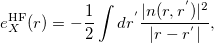
Fundamental to the XDM model is the calculation of the norm of the dipole moment of the exchange hole at a given point:

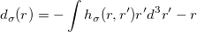$\begin{equation} d_{\sigma }(r)=-\int h_{\sigma }(r,r^{\prime })r^{\prime }d^{3}r^{\prime }-r \end{equation}$

(4.57)

where $\sigma$ labels the spin and $h_{\sigma }(r,r^{\prime })$ is the exchange-hole function. The XDM version that is implemented in Q-Chem employs the Becke-Roussel (BR) model exchange-hole function. It was not given in an analytical form and one had to determine its value at each grid point numerically. Q-Chem has developed for the first time an analytical expression for this function based on non-linear interpolation and spline techniques, which greatly improves efficiency as well as the numerical stability [30].

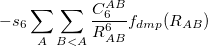
There are two different damping functions used in the XDM model of Becke and Johnson. One of them uses only the intermolecular C6 dispersion coefficient. In its Q-Chem implementation it is denoted as "XDM6". In this version the dispersion energy is computed as

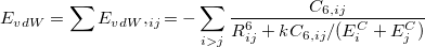$\begin{equation} E_{vdW}=\sum E_{vdW},_{ij}=-\sum _{i>j}\frac{C_{6,ij}}{R_{ij}^{6} +kC_{6,ij}/(E_{i}^{C}+E_{j}^{C})} \end{equation}$

(4.58)

where $k$ is a universal parameter, $R_{ij}^{{}}$ is the distance between atoms $i$ and $j$ , and $E_{ij}^{C}$ is the sum of the absolute values of the correlation energy of free atoms $i$ and $j$ . The dispersion coefficients $C_{6,ij}$ is computed as

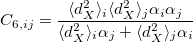$\begin{equation} C_{6,ij}=\frac{\langle d_{X}^{2}\rangle _{i}\langle d_{X}^{2}\rangle _{j} \alpha _{i}\alpha _{j}}{\langle d_{X}^{2}\rangle _{i}\alpha _{j}+\langle d_{X} ^{2}\rangle _{j}\alpha _{i}} \end{equation}$

(4.59)

where $\langle d_{X}^{2}\rangle _{i}$ is the exchange hole dipole moment of the atom, and $\alpha _{i}$ is the effective polarizability of the atom $i$ in the molecule.

The XDM6 scheme is further generalized to include higher-order dispersion coefficients, which leads to the “XDM10” model in Q-Chem implementation. The dispersion energy damping function used in XDM10 is

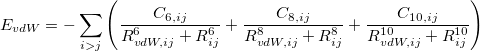$\begin{equation} E_{vdW}=-\sum _{i>j}\left(\frac{C_{6,ij}}{R_{vdW,ij}^{6}+R_{ij}^{6}}+\frac{C_{8,ij}}{R_{vdW,ij}^{8}+R_{ij}^{8}}+\frac{C_{10,ij}}{R_{vdW,ij}^{10} +R_{ij}^{10}}\right) \end{equation}$

(4.60)

where $C_{6,ij}$ , $C_{8,ij}$ and $C_{10,ij}$ are dispersion coefficients computed at higher-order multipole (including dipole, quadrupole and octopole) moments of the exchange hole [138]. In above, $R_{vdW,ij}^{{}}$ is the sum of the effective vdW radii of atoms $i$ and $j$ , which is a linear function of the so called critical distance $R_{C,ij}^{{}}$ between atoms $i$ and $j$ :

$\begin{equation} R_{vdW,ij}^{{}}=a_{1}R_{C,ij}^{{}}+a_{2} \end{equation}$

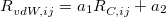(4.61)

The critical distance, $R_{C,ij}^{{}}$ , is computed by averaging these three distances:

$\begin{equation} R_{C,ij}^{{}} = \frac{1}{3}\left[ \left(\frac{C_{8,ij}}{C_{6,ij}}\right)^{1/2} +\left(\frac{C_{10,ij}}{C_{6,ij}}\right)^{1/4} +\left(\frac{C_{10,ij}}{C_{8,ij}}\right)^{1/2} \right] \end{equation}$

(4.62)

In the XDM10 scheme there are two universal parameters, $a_{1}$ and $a_{2}$ . Their default values of 0.83 and 1.35, respectively, are due to Johnson and Becke [136], determined by least square fitting to the binding energies of a set of intermolecular complexes. Please keep in mind that these values are not the only possible optimal set to use with XDM. Becke’s group has suggested later on several other XC functional combinations with XDM that employ different $a_{1}$ and $a_{2}$ values. The user is advised to consult their recent papers for more details (e.g., Refs. Becke:2010,Kannemann:2010).

The computed vdW energy is added as a post-SCF correction. In addition, Q-Chem also has implemented the first and second nuclear derivatives of vdW energy correction in both the XDM6 and XDM10 schemes.

Listed below are a number of useful options to customize the vdW calculation based on the XDM DFT approach.

DFTVDW_JOBNUMBER

Basic vdW job control

TYPE:

INTEGER

DEFAULT:

0

OPTIONS:

0

Do not apply the XDM scheme.

1

add vdW as energy/gradient correction to SCF.

2

add VDW as a DFT functional and do full SCF (this option only works with C6 XDM formula).

RECOMMENDATION:

none

DFTVDW_METHOD

Choose the damping function used in XDM

TYPE:

INTEGER

DEFAULT:

1

OPTIONS:

1

use Becke’s damping function including C6 term only.

2

use Becke’s damping function with higher-order (C8,C10) terms.

RECOMMENDATION:

none

DFTVDW_MOL1NATOMS

The number of atoms in the first monomer in dimer calculation

TYPE:

INTEGER

DEFAULT:

0

OPTIONS:

0-NATOMS

default 0

RECOMMENDATION:

none

DFTVDW_KAI

Damping factor K for C6 only damping function

TYPE:

INTEGER

DEFAULT:

800

OPTIONS:

10-1000

default 800

RECOMMENDATION:

none

DFTVDW_ALPHA1

Parameter in XDM calculation with higher-order terms

TYPE:

INTEGER

DEFAULT:

83

OPTIONS:

10-1000

RECOMMENDATION:

none

DFTVDW_ALPHA2

Parameter in XDM calculation with higher-order terms.

TYPE:

INTEGER

DEFAULT:

155

OPTIONS:

10-1000

RECOMMENDATION:

none

DFTVDW_USE_ELE_DRV

Specify whether to add the gradient correction to the XDM energy. only valid with Becke’s C6 damping function using the interpolated BR89 model.

TYPE:

LOGICAL

DEFAULT:

1

OPTIONS:

1

use density correction when applicable (default).

0

do not use this correction (for debugging purpose)

RECOMMENDATION:

none

DFTVDW_PRINT

Printing control for VDW code

TYPE:

INTEGER

DEFAULT:

1

OPTIONS:

0 no printing.

1

minimum printing (default)

2

debug printing

RECOMMENDATION:

none

Example 4.36 Below is a sample input illustrating a frequency calculation of a vdW complex consisted of He atom and N2 molecule.


$molecule

0 1
He .0 .0 3.8
N .000000 .000000 0.546986
N .000000 .000000 -0.546986
$end

$rem
JOBTYPE       FREQ
IDERIV         2
EXCHANGE      B3LYP
!default SCF setting
INCDFT         0
SCF_CONVERGENCE   8
BASIS       6-31G*
XC_GRID           1
SCF_GUESS       SAD
!vdw parameters setting
DFTVDW_JOBNUMBER    1
DFTVDW_METHOD       1
DFTVDW_PRINT        0
DFTVDW_KAI         800
DFTVDW_USE_ELE_DRV  0
$end

One should note that the XDM option can be used in conjunction with different GGA, meta-GGA pure or hybrid functionals, even though the original implementation of Becke and Johnson was in combination with Hartree-Fock exchange, or with a specific meta-GGA exchange and correlation (the BR89 exchange and the BR94 correlation described in previous sections above). For example, encouraging results were obtained using the XDM option with the popular B3LYP [137]. Becke has found more recently that this model can be efficiently combined with the old GGA exchange of Perdew 86 (the P86 exchange option in Q-Chem), and with his hyper-GGA functional B05. Using XDM together with PBE exchange plus LYP correlation, or PBE exchange plus BR94 correlation has been also found fruitful.

4.3.8 DFT-D3 Methods

Recently, Grimme proposed DFT-D3 method [141] to improve his previous DFT-D method [73] (see Section 4.3.6). Energies and analytic gradients of DFT-D3 methods are available in Q-Chem. Grimme’s DFT-D3 method can be combined with any of the density functionals available in Q-Chem.

The total DFT-D3 energy is given by

$\begin{equation} E_{\text {DFT-D3}} = E_{\text {KS-DFT}} + E_{\rm disp} \end{equation}$

(4.63)

where $E_{\text {KS-DFT}}$ is the total energy from KS-DFT and $E_{\rm disp}$ is the dispersion correction as a sum of two- and three-body energies,

$\begin{equation} E_{\rm disp} = E^{(2)}+E^{(3)} \end{equation}$

(4.64)

DFT-D3 method can be turned on by five keywords, DFT_D, DFT_D3_S6, DFT_D3_RS6, DFT_D3_S8 and DFT_D3_3BODY.

DFT_D

Controls the application of DFT-D3 or DFT-D scheme.

TYPE:

LOGICAL

DEFAULT:

None

OPTIONS:

FALSE

(or 0) Do not apply the DFT-D3 or DFT-D scheme

EMPIRICAL_GRIMME3

dispersion correction from Grimme’s DFT-D3 method

EMPIRICAL_GRIMME

dispersion correction from Grimme (see Section 4.3.6)

EMPIRICAL_CHG

dispersion correction from Chai and Head-Gordon (see Section 4.3.6)

RECOMMENDATION:

NONE

Grimme suggested four scaling factors $s_6$ , $s_{r,6}$ , $s_8$ and $s_{r,8}$ (see Equation (4) in Ref. Grimme:2010). By fixing $s_{r,8}=1.0$ , the other three factors were optimized for several functionals (see Table IV in Ref. Grimme:2010). For example, $s_{r,6}$ of 1.217 and $s_8$ of 0.722 for PBE, 1.094 and 1.682 for BLYP, 1.261 and 1.703 for B3LYP, 1.532 and 0.862 for PW6B95, 0.892 and 0.909 for BECKE97, and 1.287 and 0.928 for PBE0; these are the Q-Chem default values of $s_{r,6}$ and $s_8$ . Otherwise, the default values of $s_6$ , $s_{r,6}$ , $s_8$ and $s_{r,8}$ are 1.0.

DFT_D3_S6

Controls the strength of dispersion corrections, $s_6$ , in Grimme’s DFT-D3 method (see Table IV in Ref. Grimme:2010).

TYPE:

INTEGER

DEFAULT:

1000

OPTIONS:

n

Corresponding to $s_6 = n/1000$ .

RECOMMENDATION:

NONE

DFT_D3_RS6

Controls the strength of dispersion corrections, s $_{r,6}$ , in the Grimme’s DFT-D3 method (see Table IV in Ref. Grimme:2010).

TYPE:

INTEGER

DEFAULT:

1000

OPTIONS:

n

Corresponding to $s_{r6} = n/1000$ .

RECOMMENDATION:

NONE

DFT_D3_S8

Controls the strength of dispersion corrections, $s_8$ , in Grimme’s DFT-D3 method (see Table IV in Ref. Grimme:2010).

TYPE:

INTEGER

DEFAULT:

1000

OPTIONS:

n

Corresponding to $s_8 = n/1000$ .

RECOMMENDATION:

NONE

DFT_D3_RS8

Controls the strength of dispersion corrections, $s_{r,8}$ , in Grimme’s DFT-D3 method (see Equation (4) in Ref. Grimme:2010).

TYPE:

INTEGER

DEFAULT:

1000

OPTIONS:

n

Corresponding to $s_{r,8} = n/1000$ .

RECOMMENDATION:

NONE

The three-body interaction term, mentioned in Ref. Grimme:2010, can also be turned on, if needed.

DFT_D3_3BODY

Controls whether the three-body interaction in Grimme’s DFT-D3 method should be applied (see Eq. (14) in Ref. Grimme:2010).

TYPE:

LOGICAL

DEFAULT:

FALSE

OPTIONS:

FALSE

(or 0) Do not apply the three-body interaction term

TRUE

Apply the three-body interaction term

RECOMMENDATION:

NONE

Example 4.37 Applications of B3LYP-D3 to a methane dimer.


$comment
Geometry optimization, followed by single-point calculations 
using a larger basis set.
$end

$molecule
0 1
C       0.000000    -0.000323     1.755803
H      -0.887097     0.510784     1.390695
H       0.887097     0.510784     1.390695
H       0.000000    -1.024959     1.393014
H       0.000000     0.001084     2.842908
C       0.000000     0.000323    -1.755803
H       0.000000    -0.001084    -2.842908
H      -0.887097    -0.510784    -1.390695
H       0.887097    -0.510784    -1.390695
H       0.000000     1.024959    -1.393014
$end

$rem
jobtype         opt
exchange        B3LYP
basis           6-31G*
DFT_D           EMPIRICAL_GRIMME3
DFT_D3_S6       1000
DFT_D3_RS6      1261
DFT_D3_S8       1703
DFT_D3_3BODY    FALSE
$end

@@@

$molecule
READ
$end

$rem
jobtype         sp
exchange        B3LYP
basis           6-311++G**
DFT_D           EMPIRICAL_GRIMME3
DFT_D3_S6       1000
DFT_D3_RS6      1261
DFT_D3_S8       1703
DFT_D3_3BODY    FALSE
$end

The $\omega$ B97X-D3 and $\omega$ M06-D3 methods are implemented in Q-Chem, which automatically set the empirically-fitted parameters of the scheme, see Section 4.3.4.4.

4.3.9 Double-Hybrid Density Functional Theory

The recent advance in double-hybrid density functional theory (DH-DFT) [41, 125, 126, 127, 101], has demonstrated its great potential for approaching the chemical accuracy with a computational cost comparable to the second-order Møller-Plesset perturbation theory (MP2). In a DH-DFT, a Kohn-Sham (KS) DFT calculation is performed first, followed by a treatment of non-local orbital correlation energy at the level of second-order Møller-Plesset perturbation theory (MP2) [128]. This MP2 correlation correction includes a a same-spin (ss) component, $E_{c}^{ss}$ , as well as an opposite-spin (os) component, $E_{c}^{os}$ , which are added to the total energy obtained from the KS-DFT calculation. Two scaling parameters, $c_{ss}$ and $c_{os}$ , are introduced in order to avoid double-counting correlation:

$\begin{equation} \label{eq:dft2a} E_{\text {DH-DFT}} = E_{\text {KS-DFT}} + c_{ss} E_{c}^{ss} + c_{os} E_{c}^{os} \end{equation}$

(4.65)

Among DH functionals, $\omega$ B97X-2 [42], a long-range corrected DH functional, is described in Section 4.3.4.3.

There are three keywords for turning on DH-DFT as below.

DH

Controls the application of DH-DFT scheme.

TYPE:

LOGICAL

DEFAULT:

FALSE

OPTIONS:

FALSE

(or 0) Do not apply the DH-DFT scheme

TRUE

(or 1) Apply DH-DFT scheme

RECOMMENDATION:

NONE

SSS_FACTOR

Controls the strength of the same-spin component of PT2 correlation energy.

TYPE:

INTEGER

DEFAULT:

0

OPTIONS:

n

Corresponding to $c_{ss} = n/1000000$ in Eq. (4.65).

RECOMMENDATION:

NONE

SOS_FACTOR

Controls the strength of the opposite-spin component of PT2 correlation energy.

TYPE:

INTEGER

DEFAULT:

0

OPTIONS:

n

Corresponding to $c_{os} = n/1000000$ in Eq. (4.65).

RECOMMENDATION:

NONE

For example, B2PLYP [73], which involves 53% Hartree-Fock exchange, 47% Becke 88 GGA exchange, 73% LYP GGA correlation and 27% PT2 orbital correlation, can be called with the following input file. The PT2 correlation energy can also be computed with the efficient resolution-of-identity (RI) methods (see Section 5.5).

Example 4.38 Applications of B2PLYP functional to LiH molecule.

$comment
Geometry optimization and frequency calculation on LiH, followed by 
single-point calculations with non-RI and RI approaches. 
$end

$molecule 
0 1 
H  
Li H 1.6 
$end 

$rem
jobtype         opt
exchange        general
correlation     mp2
basis           cc-pvtz
DH              1
SSS_FACTOR      270000       !0.27 = 270000/1000000 
SOS_FACTOR      270000       !0.27 = 270000/1000000
$end

$XC_Functional
X HF   0.53
X B    0.47
C LYP  0.73
$end

@@@

$molecule
READ
$end

$rem
jobtype         freq
exchange        general
correlation     mp2
basis           cc-pvtz
DH              1
SSS_FACTOR      270000
SOS_FACTOR      270000
$end

$XC_Functional
X HF   0.53
X B    0.47
C LYP  0.73
$end

@@@

$molecule
READ
$end

$rem
jobtype         sp
exchange        general
correlation     mp2
basis           cc-pvtz
DH              1
SSS_FACTOR      270000
SOS_FACTOR      270000
$end

$XC_Functional
X HF   0.53
X B    0.47
C LYP  0.73
$end

@@@

$molecule
READ
$end

$rem
jobtype         sp
exchange        general
correlation     rimp2
basis           cc-pvtz
aux_basis       rimp2-cc-pvtz
DH              1
SSS_FACTOR      270000
SOS_FACTOR      270000
$end

$XC_Functional
X HF   0.53
X B    0.47
C LYP  0.73
$end

A simplification of input is available for the PBE0_DH [102] and PBE0_2 [103] double hybrids from the PBE based linearly-scaled one-parameter double-hybrids, automatically setting the three keywords:

Example 4.39 Applications of PBE0_DH and PBE0_2 functionals to nitrogen molecule.

$comment
Single point calculation, non-RI approach.
PBE0_DH = PBE + 50% HF + 12.5% MP2
Could also do geometry optimization and frequencies.
$end

$molecule 
0 1 
N1  
N2 N1 1.0
$end 

$rem
jobtype         sp
exchange        PBE0_DH
correlation     mp2
basis           cc-pvtz
$end

@@@

$comment
Single point calculation, expensive non-RI approach.
PBE0_2 = PBE + 79.3701% HF + 50% MP2
Could also do geometry optimization and frequencies.
$end

$molecule 
0 1 
N1  
N2 N1 1.0
$end 

$rem
jobtype         sp
exchange        PBE0_2
correlation     rimp2
basis           cc-pvtz
aux_basis       rimp2-cc-pvtz
$end

A more detailed gist of one particular class of DH functionals, the XYG3 & XYGJ-OS functionals follows below thanks to Dr Yousung Jung who implemented these functionals in Q-Chem.

A starting point of these DH functionals is the adiabatic connection formula which provides a rigorous way to define them. One considers an adiabatic path between the fictitious noninteracting Kohn-Sham system ( $\lambda$ = 0) and the real physical system ( $\lambda$ = 1) while holding the electron density fixed at its physical state for all $\lambda$ :

$\begin{equation} \label{sung1} E_{XC} \left[\rho \right]=\int _{0}^{1}U_{XC,\lambda } \left[\rho \right]d\lambda \, , \end{equation}$

(4.66)

where $U_{XC,{\lambda }}$ is the exchange correlation potential energy at a coupling strength $\lambda$ . If one assumes a linear model of the latter:

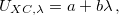$\begin{equation} \label{sung2} U_{XC,\lambda } =a+b\lambda \, , \end{equation}$

(4.67)

one obtains the popular hybrid functional that includes the Hartree-Fock exchange (or occupied orbitals) such as B3LYP. If one further uses the Gorling-Levy’s perturbation theory (GL2) to define the initial slope at $\lambda$ = 0, one obtains the doubly hybrid functional (see Eq. 4.65) that includes MP2 type perturbative terms (PT2) involving virtual Kohn-Sham orbitals:

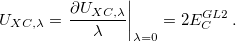$\begin{equation} \label{sung3} U_{XC,\lambda } =\left. \frac{\partial U_{XC,\lambda } }{\lambda } \right|_{\lambda =0} =2E_{C}^{GL2} \, . \end{equation}$

(4.68)

In the DH functional XYG3, as implemented in Q-Chem, the B3LYP orbitals are used to generate the density and evaluate the PT2 terms. This is different from P2PLYP, an earlier doubly hybrid functional by Grimme. P2PLYP uses truncated Kohn-Sham orbitals while XYG3 uses converged KS orbitals to evaluate the PT2 terms. The performance of XYG3 is not only comparable to that of the G3 or G2 theory for thermochemistry, but barrier heights and non-covalent interactions, including stacking interactions, are also very well described by XYG3 [101].

The recommended basis set for XYG3 is 6-311+G(3df,2p).

Due to the inclusion of PT2 terms, XYG3 or all other forms of doubly hybrid functionals formally scale as the 5th power of system size as in conventional MP2, thereby not applicable to large systems and partly losing DFT’s cost advantages. With the success of SOS-MP2 and local SOS-MP2 algorithms developed in Q-Chem, the natural extension of XYG3 is to include only opposite-spin correlation contributions, ignoring the same-spin parts. The resulting DH functional is XYGJ-OS also implemented in Q-Chem. It has 4 parameters that are optimized using thermochemistry data. This new functional is both accurate (comparable or even slightly better than XYG3) and faster. If the local algorithm is applied, the formal scaling of XYGJ-OS is cubic, without the locality, it has still 4th order scaling. Recently, XYGJ-OS becomes the only DH functional with analytical gradient [142].

Example 1: XYG3 calculation of N2. XYG3 invokes automatically the B3LYP calculation first, and use the resulting orbitals for evaluating the MP2-type correction terms. One can also use XYG3 combined with RI approximation for the PT2 terms; use EXCHANGE = XYG3RI to do so, along with an appropriate choice of auxiliary basis set.

Example 4.40 XYG3 calculation of N2


$molecule
0 1
 N     0.00000000    0.00000000    0.54777500
 N     0.00000000    0.00000000   -0.54777500
$end

$rem
 exchange   xyg3
 basis   6-311+G(3df,2p)
$end

Example 2: XYGJ-OS calculation of N2. Since it uses the RI approximation by default, one must define the auxiliary basis.

Example 4.41 XYGJ-OS calculation of N2


$molecule
0 1
 N      0.00000000    0.00000000    0.54777500
 N      0.00000000    0.00000000   -0.54777500
$end

$rem
 exchange   xygjos
 basis   6-311+G(3df,2p)
 aux_basis   rimp2-cc-pVtZ
 purecart   1111
 time_mp2   true
$end

Example 3: Local XYGJ-OS calculation of N2. The same as XYGJ-OS, except for the use of the attenuated Coulomb metric to solve the RI coefficients. Omega determines the locality of the metric.

Example 4.42 Local XYGJ-OS calculation of N2


$molecule
0 1
 N    0.000    0.000   0.54777500
 N    0.000    0.000  -0.54777500
$end

$rem
 exchange   lxygjos
 omega   200
 basis   6-311+G(3df,2p)
 aux_basis   rimp2-cc-pVtZ
 purecart   1111
$end

4.3.10 Asymptotically Corrected Exchange-Correlation Potentials

It is well known that no gradient-corrected exchange functional can simultaneously produce the correct contribution to the exchange energy density and exchange potential in the asymptotic region of molecular systems [61]. Existing GGA exchange-correlation (xc) potentials decay much faster than the correct $-1/r$ xc potential in the asymptotic region [143]. High-lying occupied orbitals and low-lying virtual orbitals are therefore too loosely bounded from these GGA functionals, and the minus HOMO energy becomes much less than the exact ionization potential (as required by the exact DFT) [144, 145]. Moreover, response properties could be poorly predicted from TDDFT calculations with GGA functionals [145]. Long-range corrected hybrid DFT (LRC-DFT), described in Section 4.3.4, has greatly remedied this situation. However, due to the use of long-range HF exchange, LRC-DFT is computationally more expensive than KS-DFT with GGA functionals.

4.3.10.1 LB94 scheme

To circumvent the above problems, van Leeuwen and Baerends proposed an asymptotically corrected (AC) exchange potential [61]:

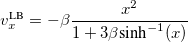$\begin{equation} v_{x}^{\text {LB}} = -\beta \frac{x^2}{1+3 \beta \mbox{sinh}^{-1}(x)} \end{equation}$

(4.69)

that will reduce to $-1/r$ , for an exponentially decaying density, in the asymptotic region of molecular systems, where $x = \frac{ \vert \nabla \rho \vert }{\rho ^{4/3}}$ is the reduced density gradient. The LB94 xc potential is formed by a linear combination of LDA xc potential and the LB exchange potential [61]:

$\begin{equation} v_{xc}^{\text {LB94}} = v_{xc}^{\text {LDA}} + v_{x}^{\text {LB}} \end{equation}$

(4.70)

The parameter $\beta$ was determined by fitting the LB94 xc potential to the beryllium atom. As mentioned in Ref. Casida:1998,Hirata:1999b, for TDDFT and TDDFT/TDA calculations, it is sufficient to include the AC xc potential for ground-state calculations followed by TDDFT calculations with an adiabatic LDA xc kernel. The implementation of LB94 xc potential in Q-Chem thus follows this; using LB94 xc potential for ground-state calculations, followed by TDDFT calculations with an adiabatic LDA xc kernel. This TDLDA/LB94 approach has been widely applied to study excited-state properties of large molecules in literature.

Since the LB exchange potential does not come from the functional derivative of some exchange functional, we use the Levy-Perdew virial relation [148] (implemented in Q-Chem) to obtain its exchange energy:

$\begin{equation} E_ x^{\text {LB}} = -\int v_ x^{\text {LB}}([\rho ],\textbf{r})[3\rho (\textbf{r})+\textbf{r}\nabla \rho (\textbf{r})]d\textbf{r} \end{equation}$

(4.71)

LB94_BETA

Set the $\beta$ parameter of LB94 xc potential

TYPE:

INTEGER

DEFAULT:

500

OPTIONS:

$n$

Corresponding to $\beta = n/10000$ .

RECOMMENDATION:

Use default, i.e., $\beta =0.05$

Example 4.43 Applications of LB94 xc potential to N $_2$ molecule.

$comment
TDLDA/LB94 calculation is performed for excitation energies.
$end

$molecule
0 1
N	0.0000	0.0000	0.0000
N	1.0977	0.0000	0.0000
$end

$rem
jobtype = sp
exchange = lb94
basis = 6-311(2+,2+)G**
cis_n_roots = 30
rpa = true
$end

4.3.10.2 LFA schemes

Another alternative, proposed by Pan, Fang and Chai [62], was to use a localized version of Fermi-Amaldi exchange-correlation functional. The resulting exchange density functional, whose functional derivative has the correct $(-1/r)$ asymptote, can be directly added to any semilocal density functional.

Three variants of this method were proposed in [62]. The simplest variant, the strictly localized Fermi-Amaldi (LFAs) scheme, is implemented in Q-Chem 4.3, for molecules consisting of atoms with $Z\leqslant 55$ .

Example 4.44 LFAs-PBE single-point TD-DFT calculation with water molecule

$comment
Use LFAs-PBE potential for ground-state calculations, followed by
TDDFT calculations with an adiabatic PBE xc kernel.
$end

$molecule
   0  1
   O
   H1  O  oh
   H2  O  oh  H1  hoh

   oh  =   1.0
   hoh = 110.0
$end.

$rem
jobtype     sp
exchange    gen
basis       6-311(2+,2+)G**
cis_n_roots 30
rpa         true
$end

$xc_functional
X PBE   1.0
C PBE   1.0
X LFAs  1.0
$end

4.3.11 Derivative discontinuity restoration scheme

From the perspective of perturbation theory, Chai and Chen proposed [149] a systematic procedure for the evaluation of the derivative discontinuity (DD) of the exchange-correlation energy functional in Kohn-Sham density functional theory, wherein the exact DD can in principle be obtained by summing up all the perturbation corrections to infinite order. Truncation of the perturbation series at low order yields an efficient scheme for obtaining the approximate DD. In particular, the first-order correction term is equivalent to the frozen-orbital approximation method.

The first-order scheme implemented in Q-Chem 4.3 supports only local or GGA functionals, does not yet support meta-GGA, HF, hybrids or non-local correlation.

FOA_FUNDGAP

Compute the frozen-orbital approximation of the fundamental gap.

TYPE:

Boolean

DEFAULT:

false

OPTIONS:

false

(default) do not compute FOA DD and fundamental gap

true

compute and print FOA fundamental gap information. Implies KS_GAP_PRINT.

RECOMMENDATION:

Use in conjuction with KS_GAP_UNIT if true.

Example 4.45 frozen-orbital approximation of DD with PBE and LFAs-PBE functionals on carbon atom

$comment
Frozen-orbital derivative discontinuity, C atom, PBE
$end

$molecule
0 3
C
$end

$rem
jobtype           sp
basis             6-31G*
method            PBE
foa_fundgap       true
ks_gap_unit       1 ! print gap info in eV
$end

@@@

$comment
with LFAs-PBE functional instead
$end

$molecule
READ
$end

$rem
jobtype           sp
basis             6-31G*
scf_guess         READ
exchange          gen
foa_fundgap       true
ks_gap_unit       1
$end

$xc_functional
X PBE  1.0
X LFAs 1.0
C PBE  1.0
$end

4.3.12 Thermally-Assisted-Occupation Density Functional Theory (TAO-DFT)

Aiming to study the ground-state properties of large strongly correlated systems with minimum computational complexity, Chai recently developed thermally-assisted-occupation density functional theory (TAO-DFT) [150]. Unlike conventional ab initio multi-reference methods, the computational complexity of TAO-DFT increases very insignificantly with the size of the active space (i.e., an active space restriction is not needed for TAO-DFT calculations), showing that TAO-DFT can be very promising for the study of large polyradical systems. In contrast to KS-DFT, TAO-DFT is a density functional theory with fractional orbital occupations produced by the Fermi-Dirac distribution (controlled by a fictitious temperature $\theta$ ). However, existing XC functionals (e.g., LDA and GGAs) in KS-DFT may also be adopted in TAO-DFT [151]. TAO-DFT has similar computational cost as KS-DFT for single-point energy calculations and analytical nuclear gradients, and reduces to KS-DFT in the absence of strong static correlation effects.

There are several $rem variables that are used for TAO-DFT.

TAO_DFT

Controls whether to use TAO-DFT.

TYPE:

Boolean

DEFAULT:

false

OPTIONS:

false

do not use TAO-DFT

true

use TAO-DFT

RECOMMENDATION:

NONE

TAO_DFT_THETA

value of $\theta$ in TAO-DFT.

TYPE:

INTEGER

DEFAULT:

7

OPTIONS:

$m$

$\theta =m\times 10^{-n}$ (hartrees), where $n$ is the value of TAO_DFT_THETA_NDP

RECOMMENDATION:

NONE

TAO_DFT_THETA_NDP

value of $\theta$ in TAO-DFT.

TYPE:

INTEGER

DEFAULT:

3

OPTIONS:

$n$

$\theta =m\times 10^{-n}$ (hartrees), where $m$ is the value of TAO_DFT_THETA

RECOMMENDATION:

NONE

Note that setting TAO_DFT_THETA=0 recovers KS-DFT [150].

In addition to the XC functional, $E_{\theta }[\rho ]$ is needed in TAO-DFT. Currently, LDA [150] and GEA (gradient expansion approximation, [151]) are available in Q-Chem.

Example 4.46 TAO-LDA calcuation on Be atom

$molecule
0 1
Be
$end
$rem
jobtype           sp
basis             6-31G*
exchange          gen
tao_dft           true
tao_dft_theta     7  ! default, theta=7 mhartree
tao_dft_theta_ndp 3  ! default
$end
$xc_functional
X   S             1.0
C   PW92          1.0
X   ETheta_LDA    1.0
$end

Example 4.47 TAO-PBE, spin-restricted calculation on stretched N $_2$

$comment
Spin-restricted calculation on stretched N2
$end
$molecule
0 1
N1
N2 N1 5
$end
$rem
jobtype           sp
basis             6-31G*
exchange          gen
tao_dft           true
tao_dft_theta     40  ! theta = 40 mhartree
tao_dft_theta_ndp 3
$end
$xc_functional
X PBE         1.0
C PBE         1.0
X ETheta_LDA  1.0
$end

Example 4.48 TAO-PBE, spin-unrestricted calculation on stretched N $_2$

$comment
Spin-unrestricted optimization calculation on stretched N2
$end
$molecule
0 1
N1
N2 N1 5
$end
$rem
jobtype           opt
unrestricted      true
basis             6-31G*
exchange          gen
tao_dft           true
tao_dft_theta     40  ! theta = 40 minihartrees
tao_dft_theta_ndp 3   ! can omit this line
scf_guess         gwh
SCF_GUESS_MIX     3   ! mix in 30% lumo in alpha to break symmetry
$end
$xc_functional
X PBE         1.0
C PBE         1.0
X ETheta_LDA  1.0
$end

ETheta_LDA may also be replaced with ETheta_GEA, see [151].

4.3.13 DFT Numerical Quadrature

In practical DFT calculations, the forms of the approximate exchange-correlation functionals used are quite complicated, such that the required integrals involving the functionals generally cannot be evaluated analytically. Q-Chem evaluates these integrals through numerical quadrature directly applied to the exchange-correlation integrand (i.e., no fitting of the XC potential in an auxiliary basis is done). Q-Chem provides a standard quadrature grid by default which is sufficient for most purposes.

The quadrature approach in Q-Chem is generally similar to that found in many DFT programs. The multi-center XC integrals are first partitioned into “atomic” contributions using a nuclear weight function. Q-Chem uses the nuclear partitioning of Becke [152], though without the atomic size adjustments". The atomic integrals are then evaluated through standard one-center numerical techniques.

Thus, the exchange-correlation energy $E_{\mathrm{XC}}$ is obtained as

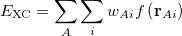$\begin{equation} \label{eq439} E_{\mathrm{XC}} =\sum \limits _ A {\sum \limits _ i {w_{Ai} f\left( {{\rm {\bf r}}_{Ai} } \right)} } \end{equation}$

(4.72)

where the first summation is over the atoms and the second is over the numerical quadrature grid points for the current atom. The $f$ function is the exchange-correlation functional. The $w_{Ai}$ are the quadrature weights, and the grid points $\ensuremath{\mathbf{r}}_{Ai}$ are given by

$\begin{equation} \label{eq440} {\rm {\bf r}}_{Ai} ={\rm {\bf R}}_ A +{\rm {\bf r}}_ i \end{equation}$

(4.73)

where $\ensuremath{\mathbf{R}}_ A$ is the position of nucleus $A$ , with the $\ensuremath{\mathbf{r}}_ i$ defining a suitable one-center integration grid, which is independent of the nuclear configuration.

The single-center integrations are further separated into radial and angular integrations. Within Q-Chem, the radial part is usually treated by the Euler-Maclaurin scheme proposed by Murry et al. [153]. This scheme maps the semi-infinite domain $[0,\infty )\to [0,1)$ and applies the extended trapezoidal rule to the transformed integrand. Recently Gill and Chien [154] proposed a radial scheme based on a Gaussian quadrature on the interval $[0,1]$ with weight function $\ln ^2x$ . This scheme is exact for integrands that are a linear combination of a geometric sequence of exponential functions, and is therefore well suited to evaluating atomic integrals. The authors refer to this scheme as MultiExp.

4.3.14 Angular Grids

Angular quadrature rules may be characterized by their degree, which is the highest degree of spherical harmonics for which the formula is exact, and their efficiency, which is the number of spherical harmonics exactly integrated per degree of freedom in the formula. Q-Chem supports the following types of angular grids:

Lebedev These are specially constructed grids for quadrature on the surface of a sphere [155, 156, 157] based on the octahedral group. Lebedev grids of the following degrees are available:

Degree	3rd	5th	7th	9th	11th	15th	17th	19th	23rd	29th
Points	6	18	26	38	50	86	110	146	194	302

Additional grids with the following number of points are also available: 74, 170, 230, 266, 350, 434, 590, 770, 974, 1202, 1454, 1730, 2030, 2354, 2702, 3074, 3470, 3890, 4334, 4802, 5294. Lebedev grids typically have efficiencies near one, with efficiencies greater than one in some cases.

Gauss-Legendre These are spherical product rules separating the two angular dimensions $\theta$ and $\phi$ . Integration in the $\theta$ dimension is carried out with a Gaussian quadrature rule derived from the Legendre polynomials (orthogonal on $[-1,1]$ with weight function unity), while the $\phi$ integration is done with equally spaced points.

A Gauss-Legendre grid is selected by specifying the total number of points, $2N^2$ , to be used for the integration. This gives a grid with $2N_{\phi }$ $\phi$ -points, $N_{\theta }$ $\theta$ -points, and a degree of $2N-1$ .

In contrast with Lebedev grids, Gauss-Legendre grids have efficiency of only 2/3 (hence more Gauss-Legendre points are required to attain the same accuracy as Lebedev). However, since Gauss-Legendre grids of general degree are available, this is a convenient mechanism for achieving arbitrary accuracy in the angular integration if desired.

Combining these radial and angular schemes yields an intimidating selection of three-dimensional quadratures. In practice, is it useful to standardize the grids used in order to facilitate the comparison of calculations at different levels of theory.

4.3.15 Standard Quadrature Grids

Both the SG-0 [158] and SG-1 [159] standard quadrature grids were designed to yield the performance of a large, accurate quadrature grid, but with as few points as possible for the sake of computational efficiency. This is accomplished by reducing the number of angular points in regions where sophisticated angular quadrature is not necessary, such as near the nuclei where the charge density is nearly spherically symmetric, while retaining large numbers of angular points in the valence region where angular accuracy is critical.

The SG-0 grid was derived in this fashion from a MultiExp-Lebedev-(23,170), (i.e., 23 radial points and 170 angular points per radial point). This grid was pruned whilst ensuring the error in the computed exchange energies for the atoms and a selection of small molecules was not larger than the corresponding error associated with SG-1. In our evaluation, the RMS error associated with the atomization energies for the molecules in the G1 data set is 72 microhartrees. While relative energies are expected to be reproduced well by this scheme, if absolute energies are being sought, a larger grid is recommended.

The SG-0 grid is implemented in Q-Chem from H to micro Hartrees, excepted He and Na; in this scheme, each atom has around 1400-point, and SG-1 is used for those their SG-0 grids have not been defined. It should be noted that, since the SG-0 grid used for H has been re-optimized in this version of Q-Chem (version 3.0), quantities calculated in this scheme may not reproduce those generated by the last version (version 2.1).

The SG-1 grid is derived from a Euler-Maclaurin-Lebedev-(50,194) grid (i.e., 50 radial points, and 194 angular points per radial point). This grid has been found to give numerical integration errors of the order of 0.2 kcal/mol for medium-sized molecules, including particularly demanding test cases such as isomerization energies of alkanes. This error is deemed acceptable since it is significantly smaller than the accuracy typically achieved by quantum chemical methods. In SG-1 the total number of points is reduced to approximately 1/4 of that of the original EML-(50,194) grid, with SG-1 generally giving the same total energies as EML-(50,194) to within a few microhartrees (0.01 kcal/mol). Therefore, the SG-1 grid is relatively efficient while still maintaining the numerical accuracy necessary for chemical reliability in the majority of applications.

Both the SG-0 and SG-1 grids were optimized so that the error in the energy when using the grid did not exceed a target threshold. For single point calculations this criterion is appropriate. However, derivatives of the energy can be more sensitive to the quality of the integration grid, and it is recommended that a larger grid be used when calculating these. Special care is required when performing DFT vibrational calculations as imaginary frequencies can be reported if the grid is inadequate. This is more of a problem with low-frequency vibrations. If imaginary frequencies are found, or if there is some doubt about the frequencies reported by Q-Chem, the recommended procedure is to perform the calculation again with a larger grid and check for convergence of the frequencies. Of course the geometry must be re-optimized, but if the existing geometry is used as an initial guess, the geometry optimization should converge in only a few cycles.

4.3.16 Consistency Check and Cutoffs for Numerical Integration

Whenever Q-Chem calculates numerical density functional integrals, the electron density itself is also integrated numerically as a test on the quality of the quadrature formula used. The deviation of the numerical result from the number of electrons in the system is an indication of the accuracy of the other numerical integrals. If the relative error in the numerical electron count reaches 0.01%, a warning is printed; this is an indication that the numerical XC results may not be reliable. If the warning appears at the first SCF cycle, it is probably not serious, because the initial-guess density matrix is sometimes not idempotent, as is the case with the SAD guess and the density matrix taken from a different geometry in a geometry optimization. If that is the case, the problem will be corrected as the idempotency is restored in later cycles. On the other hand, if the warning is persistent to the end of SCF iterations, then either a finer grid is needed, or choose an alternative method for generating the initial guess.

Users should be aware, however, of the potential flaws that have been discovered in some of the grids currently in use. Jarecki and Davidson [160], for example, have recently shown that correctly integrating the density is a necessary, but not sufficient, test of grid quality.

By default, Q-Chem will estimate the magnitude of various XC contributions on the grid and eliminate those determined to be numerically insignificant. Q-Chem uses specially developed cutoff procedures which permits evaluation of the XC energy and potential in only ${\cal {O}}({N})$ work for large molecules, where $N$ is the size of the system. This is a significant improvement over the formal ${\cal {O}}({N^3})$ scaling of the XC cost, and is critical in enabling DFT calculations to be carried out on very large systems. In very rare cases, however, the default cutoff scheme can be too aggressive, eliminating contributions that should be retained; this is almost always signaled by an inaccurate numerical density integral. An example of when this could occur is in calculating anions with multiple sets of diffuse functions in the basis. As mentioned above, when an inaccurate electron count is obtained, it maybe possible to remedy the problem by increasing the size of the quadrature grid.

Finally we note that early implementations of quadrature-based Kohn-Sham DFT employing standard basis sets were plagued by lack of rotational invariance. That is, rotation of the system yielded a significantly energy change. Clearly, such behavior is highly undesirable. Johnson et al. rectified the problem of rotational invariance by completing the specification of the grid procedure [161] to ensure that the computed XC energy is the same for any orientation of the molecule in any Cartesian coordinate system.

4.3.17 Basic DFT Job Control

For most DFT jobs two $rem variables are required: METHOD and BASIS. To request a specific pair of exchange and correlation functionals, the EXCHANGE and CORRELATION keywords can be used instead of METHOD. In addition, all of the basic input options discussed for Hartree-Fock calculations in Section 4.2.3, and the extended options discussed in Section 4.2.4 are all valid for DFT calculations. Below we list only the basic DFT-specific options (keywords).

METHOD

Specifies the exchange-correlation functional.

TYPE:

STRING

DEFAULT:

No default

OPTIONS:

NAME

Use METHOD = NAME, where NAME is

one of the DFT methods listed in Table 4.2.

RECOMMENDATION:

Consult the literature to guide your selection.

Table 4.2: Combinations of exchange and correlation density functionals and hybrid functionals accessible through the METHOD keyword.

METHOD =	Exchange	Correlation
HF	Hartree–Fock
LDA	Slater	Vosko-Wilk-Nusair parameterization #5 (VWN)
BLYP	Becke 1988 (B)	Lee-Yang-Parr (LYP)
BP86	B	Perdew 1986 (P86)
BP86-VWN	B	P86-VWN
PBE	Perdew-Burke-Ernzerhof 1996 (PBE)
PBE0	PBE hybrid with 25% HF exchange
PBE50	PBE hybrid with 50% HF exchange
B3LYP	B3LYP hybrid
BHHLYP	Modified BLYP functional with 50% HF exchange
B5050LYP	Modified B3LYP functional with 50% HF exchange
B97-D	Grimme’s modified B97 with empirical dispersion
CAM-B3LYP	Coulomb-attenuated B3LYP
X3LYP	X3LYP from Xu and Goddard
EDF1	EDF1
EDF2	EDF2
LRC-wPBE	Long-range-corrected pure PBE
LRC-wPBEH	Long-range-corrected hybrid PBE
M05	M05 hybrid
M05-2X	M05-2X hybrid
M06	M06 hybrid
M06-L	M06-L hybrid
M06-HF	M06-HF hybrid
M06-2X	M06-2X hybrid
M08-HX	M08-HX hybrid
M08-SO	M08-SO hybrid
M11	M11 long-range-corrected hybrid
M11-L	M11-L hybrid
wB97	$\omega$ B97 long-range-corrected hybrid
wB97X	$\omega$ B97X long-range-corrected hybrid
wB97X-D	$\omega$ B97X-D long-range-corrected hybrid with dispersion
	corrections
wB97X-D3	$\omega$ B97X-D3 long-range-corrected hybrid with dispersion
	corrections
wM05-D	$\omega$ M05-D long-range-corrected hybrid with dispersion
	corrections
wM06-D3	$\omega$ M06-D3 long-range-corrected hybrid with dispersion
	corrections

EXCHANGE

Specifies the exchange functional or exchange-correlation functional for hybrid.

TYPE:

STRING

DEFAULT:

No default exchange functional

OPTIONS:

NAME

Use EXCHANGE = NAME, where NAME is

one of the exchange functionals listed in Table 4.3.

RECOMMENDATION:

Consult the literature to guide your selection.

CORRELATION

Specifies the correlation functional.

TYPE:

STRING

DEFAULT:

None

No correlation.

OPTIONS:

None

No correlation

VWN

Vosko-Wilk-Nusair parameterization #5

LYP

Lee-Yang-Parr (LYP)

PW91, PW

GGA91 (Perdew-Wang)

PW92

LSDA 92 (Perdew and Wang) [46]

PK09

LSDA (Proynov-Kong) [47]

LYP(EDF1)

LYP(EDF1) parameterization

Perdew86, P86

Perdew 1986

PZ81, PZ

Perdew-Zunger 1981

PBE

Perdew-Burke-Ernzerhof 1996

TPSS

The correlation component of the TPSS functional

B94

Becke 1994 correlation in fully analytic form

B95

Becke 1995 correlation

B94hyb

Becke 1994 correlation as above, but re-adjusted for use only within

the hybrid scheme BR89B94hyb

PK06

Proynov-Kong 2006 correlation (known also as “tLap”)

(B88)OP

OP correlation [80], optimized for use with B88 exchange

(PBE)OP

OP correlation [80], optimized for use with PBE exchange

Wigner

Wigner

RECOMMENDATION:

Consult the literature to guide your selection.

Table 4.3: DFT exchange functionals available within Q-Chem.

EXCHANGE =	Description
HF	Fock exchange
Slater, S	Slater (Dirac 1930)
ETheta_LDA, ETheta_LSDA	TAO-DFT local density approximation for $E_\theta$ [150]
	(use in conjunction with another exchange functional)
ETheta_GEA	TAO-DFT gradient expansion approximation for $E_\theta$ [151]
	(use in conjunction with another exchange functional)
Becke86, B86	Becke 1986
Becke, B, B88	Becke 1988
muB88	Short-range Becke exchange, as formulated by Song et al. [114]
Gill96, Gill	Gill 1996
GG99	Gilbert and Gill, 1999
Becke(EDF1), B(EDF1)	Becke (uses EDF1 parameters)
PW86,	Perdew-Wang 1986
rPW86,	Re-fitted PW86 [51]
PW91, PW	Perdew-Wang 1991
mPW1PW91	modified PW91
mPW1LYP	modified PW91 exchange + LYP correlation
mPW1PBE	modified PW91 exchange + PBE correlation
mPW1B95	modified PW91 exchange + B97 correlation
mPWB1K	mPWB1K
PBE	Perdew-Burke-Ernzerhof 1996
AK13	Armiento and Kümmel, 2013 [63]
TPSS	The nonempirical exchange-correlation scheme of Tao,
	Perdew, Staroverov, and Scuseria (requires also that the user
	specify “TPSS” for correlation)
TPSSH	The hybrid version of TPSS (with no input line for correlation)
PBE0, PBE1PBE	PBE hybrid with 25% HF exchange
PBE50	PBE hybrid with 50% HF exchange
revPBE	revised PBE exchange [60]
PBEOP	PBE exchange + one-parameter progressive correlation
wPBE	Short-range $\omega$ PBE exchange, as formulated by Henderson et al. [115]
muPBE	Short-range $\mu$ PBE exchange, as formulated by Song et al. [114]
LRC-wPBEPBE	long-range corrected pure PBE
LRC-wPBEhPBE	long-range corrected hybrid PBE
B1B95	Becke hybrid functional with B97 correlation
B97	Becke97 XC hybrid
B97-1	Becke97 re-optimized by Hamprecht et al. (1998)
B97-2	Becke97-1 optimized further by Wilson et al. (2001)
B97-D	Grimme’s modified B97 with empirical dispersion
B3PW91, Becke3PW91, B3P	B3PW91 hybrid
B3LYP, Becke3LYP	B3LYP hybrid
B3LYP5	B3LYP based on correlation functional #5 of Vosko, Wilk,
	and Nusair (rather than their functional #3)
CAM-B3LYP	Coulomb-attenuated B3LYP
HC-O3LYP	O3LYP from Handy
X3LYP	X3LYP from Xu and Goddard
B5050LYP	modified B3LYP functional with 50% Hartree-Fock exchange
BHHLYP	modified BLYP functional with 50% Hartree-Fock exchange
B3P86	B3 exchange and Perdew 86 correlation
B3PW91	B3 exchange and GGA91 correlation
B3tLAP	Hybrid Becke exchange and PK06 correlation
HCTH	HCTH hybrid
HCTH-120	HCTH-120 hybrid
HCTH-147	HCTH-147 hybrid
HCTH-407	HCTH-407 hybrid
BOP	B88 exchange + one-parameter progressive correlation
EDF1	EDF1
EDF2	EDF2
VSXC	VSXC meta-GGA, not a hybrid
BMK	BMK hybrid
M05	M05 hybrid
M052X	M05-2X hybrid
M06L	M06-L hybrid
M06HF	M06-HF hybrid
M06	M06 hybrid
M062X	M06-2X hybrid
M08HX	M08-HX hybrid
M08SO	M08-SO hybrid
M11L	M11-L hybrid
M11	M11 long-range corrected hybrid
SOGGA	SOGGA hybrid
SOGGA11	SOGGA11 hybrid
SOGGA11X	SOGGA11-X hybrid
BR89	Becke-Roussel 1989 represented in analytic form
BR89B94h	Hybrid BR89 exchange and B94hyb correlation
omegaB97	$\omega$ B97 long-range corrected hybrid
omegaB97X	$\omega$ B97X long-range corrected hybrid
omegaB97X-D	$\omega$ B97X-D long-range corrected hybrid with dispersion
	corrections
omegaB97X-2(LP)	$\omega$ B97X-2(LP) long-range corrected double-hybrid
omegaB97X-2(TQZ)	$\omega$ B97X-2(TQZ) long-range corrected double-hybrid
MCY2	The MCY2 hyper-GGA exchange-correlation (with no
	input line for correlation)
B05	Full exact-exchange hyper-GGA functional of Becke 05 with
	RI approximation for the exact-exchange energy density
BM05	Modified B05 hyper-GGA scheme with RI approximation for
	the exact-exchange energy density used as a variable.
XYG3	XYG3 double-hybrid functional
XYGJOS	XYGJ-OS double-hybrid functional
LXYGJOS	LXYGJ-OS double-hybrid functional with localized MP2
PBE0_DH, PBE0_2	PBE double hybrid functionals, requires setting
	`CORRELATION` to an MP2 implementation
General, Gen	User defined combination of K, X and C (refer to the next
	section)

NL_CORRELATION

Specifies a non-local correlation functional that includes non-empirical dispersion.

TYPE:

STRING

DEFAULT:

None

No non-local correlation.

OPTIONS:

None

No non-local correlation

vdW-DF-04

the non-local part of vdW-DF-04

vdW-DF-10

the nonlocal part of vdW-DF-10 (aka vdW-DF2)

VV09

the nonlocal part of VV09

VV10

the nonlocal part of VV10

RECOMMENDATION:

Do not forget to add the LSDA correlation (PW92 is recommended) when using vdW-DF-04, vdW-DF-10, or VV09. VV10 should be used with PBE correlation. Choose exchange functionals carefully: HF, rPW86, revPBE, and some of the LRC exchange functionals are among the recommended choices.

NL_VV_C

Sets the parameter $C$ in VV09 and VV10. This parameter is fitted to asymptotic van der Waals $C_6$ coefficients.

TYPE:

INTEGER

DEFAULT:

89

for VV09

No default

for VV10

OPTIONS:

$n$

Corresponding to $C = n/10000$

RECOMMENDATION:

$C = 0.0093$ is recommended when a semilocal exchange functional is used. $C = 0.0089$ is recommended when a long-range corrected (LRC) hybrid functional is used. See further details in Ref. [135].

NL_VV_B

Sets the parameter $b$ in VV10. This parameter controls the short range behavior of the nonlocal correlation energy.

TYPE:

INTEGER

DEFAULT:

No default

OPTIONS:

$n$

Corresponding to $b = n/100$

RECOMMENDATION:

The optimal value depends strongly on the exchange functional used. $b = 5.9$ is recommended for rPW86. See further details in Ref. [135].

FAST_XC

Controls direct variable thresholds to accelerate exchange correlation (XC) in DFT.

TYPE:

LOGICAL

DEFAULT:

FALSE

OPTIONS:

TRUE

Turn FAST_XC on.

FALSE

Do not use FAST_XC.

RECOMMENDATION:

Caution: FAST_XC improves the speed of a DFT calculation, but may occasionally cause the SCF calculation to diverge.

XC_GRID

Specifies the type of grid to use for DFT calculations.

TYPE:

INTEGER

DEFAULT:

1

SG-1 hybrid

OPTIONS:

0

Use SG-0 for H, C, N, and O, SG-1 for all other atoms.

1

Use SG-1 for all atoms.

2

Low Quality.

$mn$

The first six integers correspond to $m$ radial points and the second six

integers correspond to $n$ angular points where possible numbers of Lebedev

angular points are listed in section 4.3.13.

$-mn$

The first six integers correspond to $m$ radial points and the second six

integers correspond to $n$ angular points where the number of Gauss-Legendre

angular points $n = 2N^2$ .

RECOMMENDATION:

Use default unless numerical integration problems arise. Larger grids may be required for optimization and frequency calculations.

XC_SMART_GRID

Uses SG-0 (where available) for early SCF cycles, and switches to the (larger) grid specified by XC_GRID (which defaults to SG-1, if not otherwise specified) for final cycles of the SCF.

TYPE:

LOGICAL

DEFAULT:

FALSE

OPTIONS:

TRUE/FALSE

RECOMMENDATION:

The use of the smart grid can save some time on initial SCF cycles.

NL_GRID

Specifies the grid to use for non-local correlation.

TYPE:

INTEGER

DEFAULT:

1

SG-1 grid

OPTIONS:

Same as for XC_GRID

RECOMMENDATION:

Use default unless computational cost becomes prohibitive, in which case SG-0 may be used. XC_GRID should generally be finer than NL_GRID.

4.3.18 Example

Example 4.49 Q-Chem input for a DFT single point energy calculation on water.

$comment
   B-LYP/STO-3G water single point calculation
$end

$molecule
   0  1
   O
   H1  O  oh
   H2  O  oh  H1  hoh

   oh  =   1.2
   hoh = 120.0
$end.

$rem
   METHOD        BLYP     Becke88 exchange + LYP correlation
   BASIS         sto-3g   Basis set
$end

4.3.19 User-Defined Density Functionals

The format for entering user-defined exchange-correlation density functionals is one line for each component of the functional. Each line requires three variables: the first defines whether the component is an exchange or correlation functional by declaring an $X$ or $C$ , respectively. The second variable is the symbolic representation of the functional as used for the EXCHANGE and CORRELATION $rem variables. The final variable is a real number corresponding to the contribution of the component to the functional. Hartree-Fock exchange contributions (required for hybrid density functionals) can be entered using only two variables ( $K$ , for HF exchange) followed by a real number.

$xc_functional
   X   exchange_symbol   coefficient
   X   exchange_symbol   coefficient
   ...
   C   correlation_symbol   coefficient
   C   correlation_symbol   coefficient
   ...
   K   coefficient
$end

Note: (1) Coefficients are real.
(2) A user-defined functional does not require all $X$ , $C$ and $K$ components.

Examples of user-defined XCs: these are XC options that for the time being can only be invoked via the user defined XC input section:

Example 4.50 Q-Chem input of water with B3tLap.

$comment
water with B3tLap
$end

$molecule
  0  1
  O
  H1  O  oh
  H2  O  oh  H1  hoh
  oh  =   0.97
  hoh = 120.0
$end

$rem
   EXCHANGE    gen 
   CORRELATION  none 
   XC_GRID   000120000194  ! recommended for high accuracy
   BASIS     G3LARGE       ! recommended for high accuracy
   THRESH   14             ! recommended for high accuracy and better convergence
$end

$xc_functional
X    Becke     0.726
X    S         0.0966
C    PK06      1.0
K    0.1713
$end

Example 4.51 Q-Chem input of water with BR89B94hyb.

$comment
water with BR89B94hyb
$end

$molecule
   0  1
   O
   H1  O  oh
   H2  O  oh  H1  hoh
   oh  =   0.97
   hoh = 120.0
$end

$rem
   EXCHANGE    gen
   CORRELATION  none
   XC_GRID   000120000194  ! recommended for high accuracy
   BASIS     G3LARGE       ! recommended for high accuracy
   THRESH   14             ! recommended for high accuracy and better convergence
$end

$xc_functional
 X    BR89      0.846
 C    B94hyb    1.0
 K              0.154
$end

More specific is the use of the RI-B05 and RI-PSTS functionals. In this release we offer only single-point SCF calculations with these functionals. Both options require a converged LSD or HF solution as initial guess, which greatly facilitates the convergence. It also requires specifying a particular auxiliary basis set:

Example 4.52 Q-Chem input of H $_2$ using RI-B05.

$comment
H2, example of SP RI-B05.
First do a well-converged LSD, G3LARGE is the basis of choice 
for good accuracy. The input lines
purecar 222
SCF_GUESS   CORE
are obligatory for the time being here.
$end

$molecule
0 1
H   0.  0.   0.0
H   0.  0.   0.7414
$end

$rem
JOBTYPE     SP
SCF_GUESS  CORE
METHOD LDA
BASIS    G3LARGE
purcar 222
THRESH    14
MAX_SCF_CYCLES   80
PRINT_INPUT     TRUE
INCDFT    FALSE
XC_GRID 000128000302
SYM_IGNORE    TRUE
SYMMETRY      FALSE
SCF_CONVERGENCE   9
$end

@@@@

$comment
For the time being the following input lines are obligatory:
purcar 22222
AUX_BASIS riB05-cc-pvtz
dft_cutoffs 0
1415 1
MAX_SCF_CYCLES   0
JOBTYPE  SP
$end

$molecule
READ
$end

$rem
JOBTYPE    SP
SCF_GUESS  READ
EXCHANGE B05 
! EXCHANGE PSTS     ! use this line for RI-PSTS
purcar 22222
BASIS G3LARGE
AUX_BASIS riB05-cc-pvtz  ! The aux basis for RI-B05 and RI-PSTS
THRESH    14
PRINT_INPUT     TRUE
INCDFT    FALSE
XC_GRID 000128000302
SYM_IGNORE    TRUE
SYMMETRY      FALSE
MAX_SCF_CYCLES   0
dft_cutoffs 0
1415 1
$end

Besides post-LSD, the RI-B05 option can be used as post-Hartree-Fock method as well, in which case one first does a well-converged HF calculation and uses it as a guess read in the consecutive RI-B05 run.

FALSE	(or 0) Do not apply long-range correction.
TRUE	(or 1) Use the long-range-corrected version of the requested functional.

FALSE	(or 0) Do not apply the DFT-D or DFT-D3 scheme
EMPIRICAL_GRIMME	dispersion correction from Grimme
EMPIRICAL_CHG	dispersion correction from Chai and Head-Gordon
EMPIRICAL_GRIMME3	dispersion correction from Grimme’s DFT-D3 method
	(see Section 4.3.8)

0	Do not apply the XDM scheme.
1	add vdW as energy/gradient correction to SCF.
2	add VDW as a DFT functional and do full SCF (this option only works with C6 XDM formula).

1	use Becke’s damping function including C6 term only.
2	use Becke’s damping function with higher-order (C8,C10) terms.

1	use density correction when applicable (default).
0	do not use this correction (for debugging purpose)

FALSE	(or 0) Do not apply the DFT-D3 or DFT-D scheme
EMPIRICAL_GRIMME3	dispersion correction from Grimme’s DFT-D3 method
EMPIRICAL_GRIMME	dispersion correction from Grimme (see Section 4.3.6)
EMPIRICAL_CHG	dispersion correction from Chai and Head-Gordon (see Section 4.3.6)

FALSE	(or 0) Do not apply the three-body interaction term
TRUE	Apply the three-body interaction term

FALSE	(or 0) Do not apply the DH-DFT scheme
TRUE	(or 1) Apply DH-DFT scheme

false	(default) do not compute FOA DD and fundamental gap
true	compute and print FOA fundamental gap information. Implies KS_GAP_PRINT.

NAME	Use METHOD = NAME, where NAME is
	one of the DFT methods listed in Table 4.2.

NAME	Use EXCHANGE = NAME, where NAME is
	one of the exchange functionals listed in Table 4.3.

None	No correlation
VWN	Vosko-Wilk-Nusair parameterization #5
LYP	Lee-Yang-Parr (LYP)
PW91, PW	GGA91 (Perdew-Wang)
PW92	LSDA 92 (Perdew and Wang) [46]
PK09	LSDA (Proynov-Kong) [47]
LYP(EDF1)	LYP(EDF1) parameterization
Perdew86, P86	Perdew 1986
PZ81, PZ	Perdew-Zunger 1981
PBE	Perdew-Burke-Ernzerhof 1996
TPSS	The correlation component of the TPSS functional
B94	Becke 1994 correlation in fully analytic form
B95	Becke 1995 correlation
B94hyb	Becke 1994 correlation as above, but re-adjusted for use only within
	the hybrid scheme BR89B94hyb
PK06	Proynov-Kong 2006 correlation (known also as “tLap”)
(B88)OP	OP correlation [80], optimized for use with B88 exchange
(PBE)OP	OP correlation [80], optimized for use with PBE exchange
Wigner	Wigner

None	No non-local correlation
vdW-DF-04	the non-local part of vdW-DF-04
vdW-DF-10	the nonlocal part of vdW-DF-10 (aka vdW-DF2)
VV09	the nonlocal part of VV09
VV10	the nonlocal part of VV10

0	Use SG-0 for H, C, N, and O, SG-1 for all other atoms.
1	Use SG-1 for all atoms.
2	Low Quality.
$mn$	The first six integers correspond to $m$ radial points and the second six
	integers correspond to $n$ angular points where possible numbers of Lebedev
	angular points are listed in section 4.3.13.
$-mn$	The first six integers correspond to $m$ radial points and the second six
	integers correspond to $n$ angular points where the number of Gauss-Legendre
	angular points $n = 2N^2$ .