5.7 DFT Methods for van der Waals Interactions
This section describes five different procedures for obtaining a better description of dispersion (van der Waals) interactions in DFT calculations: non-local correlation functionals (Section 5.7.1), empirical atom–atom dispersion potentials (“DFT-D”, Section 5.7.2), the Becke-Johnson exchange-dipole model (XDM, Section 5.7.3), the Tkatchenko-Scheffler van der Waals method (TS-vdW, Section 5.7.4), and finally the many-body dispersion method (MBD, Section 5.7.5).
5.7.1 Non-Local Correlation (NLC) Functionals
From the standpoint of the electron density, the vdW interaction is a non-local one: even for two non-overlapping, spherically-symmetric charge densities (two argon atoms, say), the presence of molecule B in the non-covalent A B complex induces ripples in the tail of A’s charge distribution, which are the hallmarks of non-covalent interactions.[Contreras-Garc
 a et al.(2011)Contreras-Garca, Johnson, Keinan, Chaudret, Piquemal, Beratan, and Yang] (This is the fundamental idea behind the non-covalent interaction plots described in Section 11.5.5; the vdW interaction manifests as large density gradients in regions of space where the density itself is small.) Semi-local GGAs that depend only on the density and its gradient cannot describe this long-range, correlation-induced interaction, and meta-GGAs at best describe it at middle-range via the Laplacian of the density and/or the kinetic energy density. A proper description of long-range electron correlation requires a non-local functional, i.e., an exchange-correlation potential having the form
 |
(5.26) |
In this way, a perturbation at a point  (due to B, say) then induces an exchange-correlation potential at a (possibly far-removed) point
  (on A).
Q-Chem includes four such functionals that can describe dispersion interactions:
vdW-DF-04, developed by Langreth, Lundqvist, and coworkers,[Dion et al.(2004)Dion, Rydberg, Schröder, Langreth, and Lundqvist, Dion et al.(2005)Dion, Rydberg, Schröder, Langreth, and Lundqvist] implemented as described in Ref. Vydrov:2008.
vdW-DF-10 (also known as vdW-DF2), which is a re-parameterization of vdW-DF-04.[Lee et al.(2010)Lee, Murray, Kong, Lundqvist, and Langreth]
VV09, developed[Vydrov and Van Voorhis(2009)] and implemented[Vydrov and Van Voorhis(2010a)] by Vydrov and Van Voorhis.
VV10 by Vydrov and Van Voorhis.[Vydrov and Van Voorhis(2010b)]
rVV10 by Sabatini and coworkers.[Sabatini et al.(2013)Sabatini, Gorni, and de Gironcoli]
Each of these functionals is implemented in a self-consistent manner, and analytic gradients with respect to nuclear displacements are available.[Vydrov et al.(2008)Vydrov, Wu, and Van Voorhis, Vydrov and Van Voorhis(2010a), Vydrov and Van Voorhis(2010b)] The non-local correlation is governed by the $rem variable NL_CORRELATION, which can be set to one of the four values: vdW-DF-04, vdW-DF-10, VV09, or VV10. The vdW-DF-04, vdW-DF-10, and VV09 functionals are used in combination with LSDA correlation, which must be specified explicitly. For instance, vdW-DF-10 is invoked by the following keyword combination:
CORRELATION        PW92
NL_CORRELATION     vdW-DF-10
VV10 is used in combination with PBE correlation, which must be added explicitly. In addition, the values of two parameters,  and
and  (see Ref. Vydrov:2008), must be specified for VV10. These parameters are controlled by the $rem variables NL_VV_C and NL_VV_B, respectively. For instance, to invoke VV10 with
  and
and  , the following input is used:
CORRELATION        PBE
NL_CORRELATION     VV10
NL_VV_C            93
NL_VV_B            590
The variable NL_VV_C may also be specified for VV09, where it has the same meaning. By default,  is used in VV09 (i.e. NL_VV_C is set to 89). However, in VV10 neither nor are assigned a default value and must always be provided in the input.
Unlike local (LSDA) and semi-local (GGA and meta-GGA) functionals, for non-local functionals evaluation of the correlation energy requires a double integral over the spatial variables, as compared to the single integral [Eq. E_XC] required for semi-local functionals:
 |
(5.27) |
In practice, this double integration is performed numerically on a quadrature grid.[Vydrov et al.(2008)Vydrov, Wu, and Van Voorhis, Vydrov and Van Voorhis(2010a), Vydrov and Van Voorhis(2010b)] By default, the SG-1 quadrature (described in Section 5.5.2 below) is used to evaluate  , but a different grid can be requested via the $rem variable NL_GRID. The non-local energy is rather insensitive to the fineness of the grid such that SG-1 or even SG-0 grids can be used in most cases, but a finer grid may be required to integrate other components of the functional. This is controlled by the XC_GRID variable discussed in Section 5.5.2.
The two functionals originally developed by Vydrov and Van Voorhis can be requested by specifying METHOD = VV10 or METHOD LC-VV10. In addition, the combinatorially-optimized functionals of Mardirossian and Head-Gordon ( B97X-V, B97M-V, and B97M-V) make use of non-local correlation and can be invoked by setting METHOD to wB97X-V, B97M-V, or wB97M-V.
Example 5.51 Geometry optimization of the methane dimer using VV10 with rPW86 exchange.
$molecule
   0 1
   C   0.000000  -0.000140   1.859161
   H  -0.888551   0.513060   1.494685
   H   0.888551   0.513060   1.494685
   H   0.000000  -1.026339   1.494868
   H   0.000000   0.000089   2.948284
   C   0.000000   0.000140  -1.859161
   H   0.000000  -0.000089  -2.948284
   H  -0.888551  -0.513060  -1.494685
   H   0.888551  -0.513060  -1.494685
   H   0.000000   1.026339  -1.494868
$end

$rem
   JOBTYPE            opt
   BASIS              aug-cc-pVTZ
   EXCHANGE           rPW86
   CORRELATION        PBE
   XC_GRID            2
   NL_CORRELATION     VV10
   NL_GRID            1
   NL_VV_C            93
   NL_VV_B            590
$end
In the above example, the SG-2 grid is used to evaluate the rPW86 exchange and PBE correlation, but a coarser SG-1 grid is used for the non-local part of VV10. Furthermore, the above example is identical to specifying METHOD = VV10.
NL_CORRELATION
Specifies a non-local correlation functional that includes non-empirical dispersion.
TYPE:
STRING
DEFAULT:
None
No non-local correlation.
OPTIONS:
None
No non-local correlation
vdW-DF-04
the non-local part of vdW-DF-04
vdW-DF-10
the non-local part of vdW-DF-10 (also known as vdW-DF2)
VV09
the non-local part of VV09
VV10
the non-local part of VV10
RECOMMENDATION:
Do not forget to add the LSDA correlation (PW92 is recommended) when using vdW-DF-04, vdW-DF-10, or VV09. VV10 should be used with PBE correlation. Choose exchange functionals carefully: HF, rPW86, revPBE, and some of the LRC exchange functionals are among the recommended choices.
NL_VV_C
Sets the parameter
coefficients.
TYPE:
INTEGER
DEFAULT:
89
for VV09
No default
for VV10
OPTIONS:

Corresponding to

RECOMMENDATION:
NL_VV_B
Sets the parameter
TYPE:
INTEGER
DEFAULT:
No default
OPTIONS:
Corresponding to
RECOMMENDATION:
The optimal value depends strongly on the exchange functional used.
USE_RVV10
Used to turn on the rVV10 NLC functional
TYPE:
LOGICAL
DEFAULT:
FALSE
OPTIONS:
FALSE
Use VV10 NLC (the default for NL_CORRELATION)
TRUE
Use rVV10 NLC
RECOMMENDATION:
Set to TRUE if the rVV10 NLC is desired.
5.7.2 Empirical Dispersion Corrections: DFT-D
A major development in DFT during the mid-2000s was the recognition that, first of all, semi-local density functionals do not properly capture dispersion (van der Waals) interactions, a problem that has been addressed only much more recently by the non-local correlation functionals discussed in Section 5.7.1; and second, that a cheap and simple solution to this problem is to incorporate empirical potentials of the form  , where the coefficients are pairwise atomic parameters. This approach, which is an alternative to the use of a non-local correlation functional, is known as dispersion-corrected DFT (DFT-D).[Grimme(2011), Grimme et al.(2016)Grimme, Hansen, Brandenburg, and Bannwarth]
There are currently three unique DFT-D methods in Q-Chem. These are requested via the $rem variable DFT_D and are discussed below.
DFT_D
Controls the empirical dispersion correction to be added to a DFT calculation.
TYPE:
LOGICAL
DEFAULT:
None
OPTIONS:
FALSE
(or 0) Do not apply the DFT-D2, DFT-CHG, or DFT-D3 scheme
EMPIRICAL_GRIMME
DFT-D2 dispersion correction from Grimme[Grimme(2006b)]
EMPIRICAL_CHG
DFT-CHG dispersion correction from Chai and Head-Gordon[Chai and Head-Gordon(2008b)]
EMPIRICAL_GRIMME3
DFT-D3(0) dispersion correction from Grimme (deprecated as
of Q-Chem 5.0)
D3_ZERO
DFT-D3(0) dispersion correction from Grimme et al.[Grimme et al.(2010)Grimme, Antony, Ehrlich, and Krieg]
D3_BJ
DFT-D3(BJ) dispersion correction from Grimme et al.[Grimme et al.(2011)Grimme, Ehrlich, and Goerigk]
D3_CSO
DFT-D3(CSO) dispersion correction from Schröder et al.[Schröder et al.(2015)Schröder, Creon, and Schwabe]
D3_ZEROM
DFT-D3M(0) dispersion correction from Smith et al.[Smith et al.(2016)Smith, Burns, Patkowski, and Sherrill]
D3_BJM
DFT-D3M(BJ) dispersion correction from Smith et al.[Smith et al.(2016)Smith, Burns, Patkowski, and Sherrill]
D3_OP
DFT-D3(op) dispersion correction from Witte et al.[Witte et al.(2017a)Witte, Mardirossian, Neaton, and Head-Gordon]
D3
Automatically select the "best" available D3 dispersion correction
RECOMMENDATION:
Use the D3 option, which selects the empirical potential based on the density functional specified by the user.
The oldest of these approaches is DFT-D2,[Grimme(2006b)] in which the empirical dispersion potential has the aforementioned form, namely, pairwise atomic  terms:
 |
(5.28) |
This function is damped at short range, where 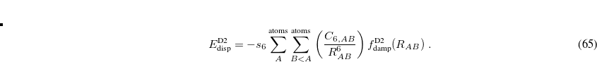 diverges, via
![\begin{equation} f^{\text {D2}}_{\text {damp}}(R_{AB}) = \left[1+e^{-d(R_{AB}/R_{0,AB} - 1)}\right]^{-1} \end{equation}](images/img-0417.png) |
(5.29) |
which also helps to avoid double-counting of electron correlation effects, since short- to medium-range correlation is included via the density functional. (The quantity  is the sum of the van der Waals radii for atoms
  and
and  , and
, and  is an additional parameter.) The primary parameters in Eq. eqn:C6 are atomic coefficients
  , from which the pairwise parameters in Eq. eqn:C6 are obtained as geometric means, as is common in classical force fields:
 |
(5.30) |
The total energy in DFT-D2 is of course  .
.
DFT-D2 is available in Q-Chem including analytic gradients and frequencies, thanks to the efforts of David Sherrill’s group. The D2 correction can be used with any density functional that is available in Q-Chem, although its use with the non-local correlation functionals discussed in Section 5.7.1 seems inconsistent and is not recommended. The global parameter  in Eq. eqn:C6 was optimized by Grimme for four different functionals,[Grimme(2006b)] and Q-Chem uses these as the default values:
  for PBE,
  for BLYP,
  for BP86, and for B3LYP. For all other functionals,
  by default. The D2 parameters, including the coefficients and the atomic van der Waals radii, can be modified using a $empirical_dispersion input section. For example:
$empirical_dispersion
   S6 1.1
   D 10.0
   C6 Ar 4.60 Ne 0.60
   VDW_RADII Ar 1.60 Ne 1.20
$end
Values not specified explicitly default to the values optimized by Grimme.
Note: (i) DFT-D2 is only defined for elements up to Xe.
(ii) B97-D is an exchange-correlation functional that automatically employs the DFT-D2 dispersion correction when used via METHOD = B97-D.
An alternative to Grimme’s DFT-D2 is the empirical dispersion correction of Chai and Head-Gordon,[Chai and Head-Gordon(2008b)] which uses the same form as Eq. eqn:C6 but with a slightly different damping function:
![$\displaystyle \label{eqn:CHG} f^{\text {CHG}}_{\text {damp}}(R_{AB}) = \bigl [1+a(R_{AB}/R_{0,AB})^{-12}\bigr ]^{-1} $](images/img-0427.png) |
(5.31) |
This version is activated by setting DFT_D = EMPIRICAL_CHG, and the damping parameter  is controlled by the keyword DFT_D_A.
DFT_D_A
Controls the strength of dispersion corrections in the Chai–Head-Gordon DFT-D scheme, Eq. eqn:CHG.
TYPE:
INTEGER
DEFAULT:
600
OPTIONS:
Corresponding to
.
RECOMMENDATION:
Use the default.
Note: (i) DFT-CHG is only defined for elements up to Xe.
(ii) The B97X-D and M05-D functionals automatically employ the DFT-CHG dispersion correction when used via METHOD = wB97X-D or wM05-D.
Grimme’s more recent DFT-D3 method[Grimme et al.(2010)Grimme, Antony, Ehrlich, and Krieg] constitutes an improvement on his D2 approach, and is also available along with analytic first and second derivatives, for any density functional that is available in Q-Chem. The D3 correction includes a potential akin to that in D2 but including atomic  terms as well:
![\begin{equation} \label{eq:D3eqn} E_{\text {D3,2-body}} = - \sum ^{\text {atoms}}_ A\sum ^{\text {atoms}}_{B<A} \left[ s_6\left(\frac{C_{6,AB}}{R_{AB}^6}\right) f_{\text {damp,6}}(R_{AB}) +s_8\left(\frac{C_{8,AB}}{R_{AB}^8}\right) f_{\text {damp,8}}(R_{AB}) \right] \; . \end{equation}](images/img-0430.png) |
(5.32) |
The total D3 dispersion correction consists of this plus a three-body term of the Axilrod-Teller-Muto (ATM) triple-dipole variety, so that the total D3 energy is 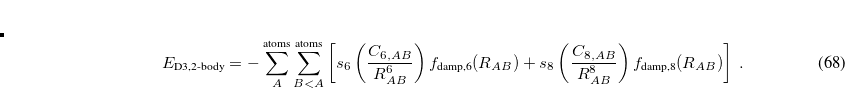
Several versions of DFT-D3 are available as of Q-Chem 5.0, which differ in the choice of the two damping functions. Grimme’s formulation,[Grimme et al.(2010)Grimme, Antony, Ehrlich, and Krieg] which is now known as the “zero-damping” version [DFT-D3(0)], uses damping functions of the form
![\begin{equation} \label{eq:zero-damping} f_{\text {damp},n}^{\text {D3(0)}}(R_{AB}) = \left[1+6\left(\frac{R_{AB}}{s_{r,n}R_{0,AB}}\right)^{-\beta _ n}\right]^{-1} \end{equation}](images/img-0432.png) |
(5.33) |
for 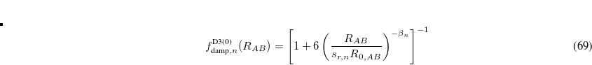 or 8,
or 8,  , and
, and  . The parameters come from atomic van der Waals radii,
  is a functional-dependent parameter, and
  . Typically is set to unity and
  is optimized for the functional in question.
The more recent Becke–Johnson-damping version of DFT-D3,[Grimme et al.(2011)Grimme, Ehrlich, and Goerigk] DFT-D3(BJ), is designed to be finite (but non-zero) as  . The damping functions used in DFT-D3(BJ) are
 |
(5.34) |
where  and
and  are adjustable parameters fit for each density functional. As in DFT-D3(0), is generally fixed to unity and is optimized for each functional. DFT-D3(BJ) generally outperforms the original DFT-D3(0) version.[Grimme et al.(2011)Grimme, Ehrlich, and Goerigk]
The -only (CSO) approach of Schröder et al.[Schröder et al.(2015)Schröder, Creon, and Schwabe] discards the term in Eq. eq:D3eqn and uses a damping function with one parameter, :
![\begin{equation} \label{eq:cso-damping} f_{\text {damp},6}^{\text {D3(CSO)}}(R_{AB}) = \frac{C_{AB}^6}{R_{AB}^6+(2.5\mbox{\AA })^6} \left(s_6+\frac{\alpha ^{}_1}{1 + \exp [R_{AB}-(2.5\mbox{\AA }) R_{0,AB}]}\right) \; . \end{equation}](images/img-0443.png) |
(5.35) |
The DFT-D3(BJ) approach was re-parameterized by Smith et al.[Smith et al.(2016)Smith, Burns, Patkowski, and Sherrill] to yield the “modified” DFT-D3(BJ) approach, DFT-D3M(BJ), whose parameterization relied heavily on non-equilibrium geometries. The same authors also introduces a modification DFT-D3M(0) of the original zero-damping correction, which introduces one additional parameter () as compared to DFT-D3(0):
![\begin{equation} \label{eq:zero-m-damping} f_{\text {damp},n}^{\text {D3M(0)}}(R_{AB}) = \left[1+6\left(\frac{R_{AB}}{s_{r,n}R_{0,AB}}+\alpha ^{}_1 R_{0,AB}\right)^{-\beta _ n}\right]^{-1}. \end{equation}](images/img-0444.png) |
(5.36) |
Finally, optimized power approach of Witte et al.[Witte et al.(2017a)Witte, Mardirossian, Neaton, and Head-Gordon] treats the exponent, 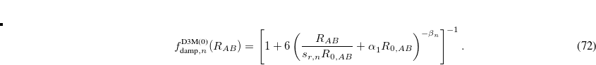 , as an optimizable parameter, given by
 |
(5.37) |
Note that 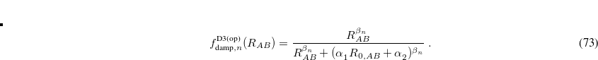 .
.
To summarize this bewildering array of D3 damping functions:
DFT-D3(0) is requested by setting DFT_D = D3_ZERO. The model depends on four scaling parameters (
, , , and  ), as defined in Eq. eq:zero-damping.
 DFT-D3(BJ) is requested by setting DFT_D = D3_BJ. The model depends on four scaling parameters (
, , , and ), as defined in Eq. eq:bj-damping. DFT-D3(CSO) is requested by setting DFT_D = D3_CSO. The model depends on two scaling parameters (
and ), as defined in Eq. eq:cso-damping. DFT-D3M(0) is requested by setting DFT_D = D3_ZEROM. The model depends on five scaling parameters (
, , , , and ), as defined in Eq. eq:zero-m-damping. DFT-D3M(BJ) is requested by setting DFT_D = D3_BJM. The model depends on four scaling parameters (
, , , and ), as defined in Eq. eq:bj-damping. DFT-D3(op) is requested by setting DFT_D = D3_OP. The model depends on four scaling parameters (
, , , , and ), as defined in Eq. eq:bj-damping.
The scaling parameters in these damping functions can be modified using the $rem variables described below. Alternatively, one may simply set DFT_D = D3, and a D3 dispersion correction will be selected automatically, if one is available for the selected functional.
Note: (i) DFT-D3(0) is defined for elements up to Pu ( ).
).
(ii) The B97-D3(0), B97X-D3, M06-D3 functionals automatically employ the DFT-D3(0) dispersion correction when invoked by setting METHOD equal to B97-D3, wB97X-D3, or wM06-D3.
(iii) The old way of invoking DFT-D3, namely through the use of EMPIRICAL_GRIMME3, is still supported, though its use is discouraged since D3_ZERO accomplishes the same thing but with additional precision for the relevant parameters.
(iv) When DFT_D = D3, parameters may not be overwritten, with the exception of DFT_D3_3BODY; this is intended as a user-friendly option. This is also the case when EMPIRICAL_GRIMME3 is employed for a functional parameterized in Q-Chem. When any of D3_ZERO, D3_BJ, etc. are chosen, Q-Chem will automatically populate the parameters with their default values, if they available for the desired functional, but these defaults can still be overwritten by the user.
DFT_D3_S6
The linear parameter
TYPE:
INTEGER
DEFAULT:
100000
OPTIONS:
Corresponding to
.
RECOMMENDATION:
NONE
DFT_D3_RS6
The nonlinear parameter
TYPE:
INTEGER
DEFAULT:
100000
OPTIONS:
Corresponding to
.
RECOMMENDATION:
NONE
DFT_D3_S8
The linear parameter
TYPE:
INTEGER
DEFAULT:
100000
OPTIONS:
Corresponding to
.
RECOMMENDATION:
NONE
DFT_D3_RS8
The nonlinear parameter
TYPE:
INTEGER
DEFAULT:
100000
OPTIONS:
Corresponding to
.
RECOMMENDATION:
NONE
DFT_D3_A1
The nonlinear parameter
TYPE:
INTEGER
DEFAULT:
100000
OPTIONS:
Corresponding to
.
RECOMMENDATION:
NONE
DFT_D3_A2
The nonlinear parameter
TYPE:
INTEGER
DEFAULT:
100000
OPTIONS:
Corresponding to
.
RECOMMENDATION:
NONE
DFT_D3_POWER
The nonlinear parameter
TYPE:
INTEGER
DEFAULT:
600000
OPTIONS:
Corresponding to
.
RECOMMENDATION:
NONE
The three-body interaction term,  ,[Grimme et al.(2010)Grimme, Antony, Ehrlich, and Krieg] must be explicitly turned on, if desired.
DFT_D3_3BODY
Controls whether the three-body interaction in Grimme’s DFT-D3 method should be applied (see Eq. (14) in Ref. Grimme:2010).
TYPE:
LOGICAL
DEFAULT:
FALSE
OPTIONS:
FALSE (or 0)
Do not apply the three-body interaction term
TRUE
Apply the three-body interaction term
RECOMMENDATION:
NONE
Example 5.52 Applications of B3LYP-D3(0) with custom parameters to a methane dimer.
$comment
   Geometry optimization, followed by single-point calculations using a larger
   basis set.
$end

$molecule
   0 1
   C       0.000000    -0.000323     1.755803
   H      -0.887097     0.510784     1.390695
   H       0.887097     0.510784     1.390695
   H       0.000000    -1.024959     1.393014
   H       0.000000     0.001084     2.842908
   C       0.000000     0.000323    -1.755803
   H       0.000000    -0.001084    -2.842908
   H      -0.887097    -0.510784    -1.390695
   H       0.887097    -0.510784    -1.390695
   H       0.000000     1.024959    -1.393014
$end

$rem
   JOBTYPE         opt
   EXCHANGE        B3LYP
   BASIS           6-31G*
   DFT_D           D3_ZERO
   DFT_D3_S6       100000
   DFT_D3_RS6      126100
   DFT_D3_S8       170300
   DFT_D3_3BODY    FALSE
$end

@@@

$molecule
   read
$end

$rem
   JOBTYPE         sp
   EXCHANGE        B3LYP
   BASIS           6-311++G**
   DFT_D           D3_ZERO
   DFT_D3_S6       100000
   DFT_D3_RS6      126100
   DFT_D3_S8       170300
   DFT_D3_3BODY    FALSE
$end
5.7.3 Exchange-Dipole Model (XDM)
Becke and Johnson have proposed an exchange dipole model (XDM) of dispersion.[Becke and Johnson(2005), Johnson and Becke(2005)] The attractive dispersion energy arises in this model via the interaction between the instantaneous dipole moment of the exchange hole in one molecule, and the induced dipole moment in another. This is a conceptually simple yet powerful approach that has been shown to yield very accurate dispersion coefficients without fitting parameters. This allows the calculation of both intermolecular and intramolecular dispersion interactions within a single DFT framework. The implementation and validation of this method in the Q-Chem code is described in Ref. Kong:2009.
The dipole moment of the exchange hole function  is given at point by
 |
(5.38) |
where  . This depends on a model of the exchange hole, and the implementation in Q-Chem uses the Becke-Roussel (BR) model.[Becke and Roussel(1989)] In most implementations the BR model,
  is not available in analytic form and its value must be numerically at each grid point. Q-Chem developed for the first time an analytical expression for this function,[Kong et al.(2009)Kong, Gan, Proynov, Freindorf, and Furlani] based on non-linear interpolation and spline techniques, which greatly improves efficiency as well as the numerical stability.
Two different damping functions have been used with XDM. One of them relies only the intermolecular coefficient, and its implementation in Q-Chem is denoted as “XDM6”. In this version the dispersion energy is
 |
(5.39) |
where 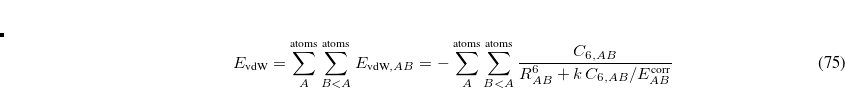 is a universal parameter, and
  is the sum of the absolute values of the correlation energies of the free atoms and . The dispersion coefficients
  is computed according to
 |
(5.40) |
where  is the square of the exchange-hole dipole moment of atom , whose effective polarizability (in the molecule) is
  .
.
The XDM6 scheme can be further generalized to include higher-order dispersion coefficients, which leads to the “XDM10” model in Q-Chem:
 |
(5.41) |
The higher-order dispersion coefficients are computed using higher-order multipole moments of the exchange hole.[Johnson and Becke(2006)] The quantity 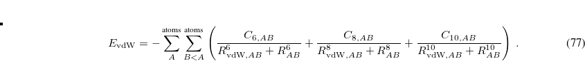 is the sum of the effective van der Waals radii of atoms and ,
 |
(5.42) |
with a critical distance
![\begin{equation} R_{{\text {crit}},AB}^{{} = \frac{1}{3}\left[ \left(\frac{C_{8,AB}}{C_{6,AB}}\right)^{1/2} +\left(\frac{C_{10,AB}}{C_{6,AB}}\right)^{1/4} +\left(\frac{C_{10,AB}}{C_{8,AB}}\right)^{1/2} \right] \; . \end{equation}](images/img-0472.png) |
(5.43) |
XDM10 contains two universal parameters, 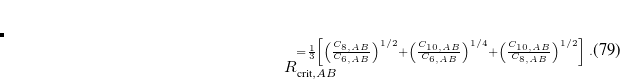 and
and  , whose default values of 0.83 and 1.35, respectively, were fit to reproduce intermolecular interaction energies.[Johnson and Becke(2005)] Becke later suggested several other XC functional combinations with XDM, which employ different values of and . The user is advised to consult the recent literature for details.[Becke and Kannemann(2010), Kannemann and Becke(2010)]
As in DFT-D, the van der Waals energy is added as a post-SCF correction. Analytic gradients and Hessians are available for both XDM6 and XDM10. Additional job control and customization options are listed below.
DFTVDW_JOBNUMBER
Basic vdW job control
TYPE:
INTEGER
DEFAULT:
0
OPTIONS:
0
Do not apply the XDM scheme.
1
Add vdW as energy/gradient correction to SCF.
2
Add vDW as a DFT functional and do full SCF (this option only works with XDM6).
RECOMMENDATION:
None
DFTVDW_METHOD
Choose the damping function used in XDM
TYPE:
INTEGER
DEFAULT:
1
OPTIONS:
1
Use Becke’s damping function including
2
Use Becke’s damping function with higher-order (
) terms.
RECOMMENDATION:
None
DFTVDW_MOL1NATOMS
The number of atoms in the first monomer in dimer calculation
TYPE:
INTEGER
DEFAULT:
0
OPTIONS:
0–

RECOMMENDATION:
None
DFTVDW_KAI
Damping factor
TYPE:
INTEGER
DEFAULT:
800
OPTIONS:
10–1000
RECOMMENDATION:
None
DFTVDW_ALPHA1
Parameter in XDM calculation with higher-order terms
TYPE:
INTEGER
DEFAULT:
83
OPTIONS:
10-1000
RECOMMENDATION:
None
DFTVDW_ALPHA2
Parameter in XDM calculation with higher-order terms.
TYPE:
INTEGER
DEFAULT:
155
OPTIONS:
10-1000
RECOMMENDATION:
None
DFTVDW_USE_ELE_DRV
Specify whether to add the gradient correction to the XDM energy. only valid with Becke’s
TYPE:
LOGICAL
DEFAULT:
1
OPTIONS:
1
Use density correction when applicable.
0
Do not use this correction (for debugging purposes).
RECOMMENDATION:
None
DFTVDW_PRINT
Printing control for VDW code
TYPE:
INTEGER
DEFAULT:
1
OPTIONS:
0
No printing.
1
Minimum printing (default)
2
Debug printing
RECOMMENDATION:
None
Example 5.53 Sample input illustrating a frequency calculation of a vdW complex consisted of He atom and N molecule.
$molecule
   0 1
   He 0.000000  0.00000   3.800000
   N  0.000000  0.000000  0.546986
   N  0.000000  0.000000 -0.546986
$end

$rem
   JOBTYPE             FREQ
   IDERIV              2
   EXCHANGE            B3LYP
   INCDFT              0
   SCF_CONVERGENCE     8
   BASIS               6-31G*
   !vdw parameters settings
   DFTVDW_JOBNUMBER    1
   DFTVDW_METHOD       1
   DFTVDW_PRINT        0
   DFTVDW_KAI          800
   DFTVDW_USE_ELE_DRV  0
$end
The original XDM implementation by Becke and Johnson used Hartree-Fock exchange but XDM can be used in conjunction with GGA, meta-GGA, or hybrid functionals, or with a specific meta-GGA exchange and correlation (the BR89 exchange and BR94 correlation functionals, for example). Encouraging results have been obtained using XDM with B3LYP.[Kong et al.(2009)Kong, Gan, Proynov, Freindorf, and Furlani] Becke has found more recently that this model can be efficiently combined with the P86 exchange functional, with the hyper-GGA functional B05. Using XDM together with PBE exchange plus LYP correlation, or PBE exchange plus BR94 correlation, has been also found fruitful. See Refs. Kannemann:2010 and Otero-de-la-Roza:2013 for some recent choices in this regard.
5.7.4 Tkatchenko-Scheffler van der Waals Model (TS-vdW)
Tkatchenko and Scheffler[Tkatchenko and Scheffler(2009)] have developed a pairwise method for van der Waals (vdW, i.e., dispersion) interactions, based on a scaling approach that yields in situ atomic polarizabilities ( ), dispersion coefficients (), and vdW radii (
 ) that reflect to the local electronic environment, based on scaling the free-atom values of these parameters in order to account for how the volume of a given atom is modified by its molecular environment. The size of an atom in a molecule is determined using the Hirshfeld partition of the electron density. (Hirshfeld or “stockholder” partitioning, which also affords one measure of atomic charges in a molecule, is described in Section 11.2.1). In the resulting “TS-vdW” approach, only a single empirical range-separation parameter (
 ) is required, which depends upon the underlying exchange-correlation functional.
Note: The parameter is currently implemented only for the PBE, PBE0, BLYP, B3LYP, revPBE, M06L, and M06 functionals.
The TS-vdW energy expression is based on a pairwise-additive model for the dispersion energy,
 |
(5.44) |
As in DFT-D the 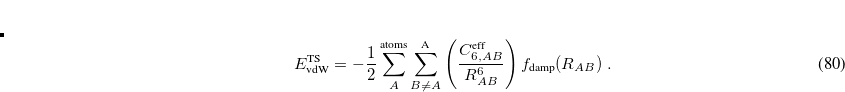 potentials in Eq. eq:ts_energy must be damped at short range, and the TS-vdW model uses the damping function
![\begin{equation} \label{eq:fdamp_ TS-vdW} f_{\text {damp}}(R_{AB}) = \frac{1}{ 1+\exp \bigl [-d (R_{AB}/s^{}_ R R_{\mathrm{vdW,}AB}^{\text {eff}} - 1)\bigr ] } \end{equation}](images/img-0481.png) |
(5.45) |
with  and an empirical parameter that is optimized in a functional-specific way to reproduce intermolecular interaction energies.[Tkatchenko and Scheffler(2009)] Optimized values for several different functionals are listed in Table 5.4.
PBE |
PBE0 |
BLYP |
B3LYP |
revPBE |
M06L |
M06 |
|
|
0.94 |
0.96 |
0.62 |
0.84 |
0.60 |
1.26 |
1.16 |
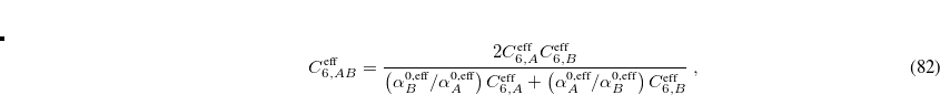
The pairwise coefficients  in Eq. eq:ts_energy are constructed from the corresponding atomic parameters
  via
via
 |
(5.46) |
as opposed to the simple geometric mean that is used for parameters in the empirical DFT-D methods [Eq. eq:C_6AB]. These are “effective” coefficients in the sense that they account for the local electronic environment. As indicated above, this is accomplished by scaling the corresponding free-atom values, i.e.,
 |
(5.47) |
where  is the effective volume of atom in the molecule, as determined using Hirshfeld partitioning. Effective atomic polarizabilities and vdW radii are obtained analogously:
 |
(5.48) |
 |
(5.49) |
All three of these atom-specific parameters are therefore functionals of the electron density.
As with DFT-D, the cost to evaluate the dispersion correction in Eq. eq:ts_energy is essentially zero in comparison to the cost of a DFT calculation. A recent review[Hermann et al.(2017)Hermann, DiStasio Jr., and Tkatchanko] shows that the performance of the TS-vdW model is on par with that of other pairwise dispersion corrections. For example, for intermolecular interaction energies in the S66 data set,[Řezáč et al.(2011)Řezáč, Riley, and Hobza] the TS-vdW correction added to PBE affords a mean absolute error of 0.4 kcal/mol and a maximum error of 1.5 kcal/mol, whereas the corresponding errors for PBE alone are 2.2 kcal/mol (mean) and 7.2 kcal/mol (maximum).
During the implementation of the TS-vdW scheme in Q-Chem, it was noted that evaluation of the free-atom volumes affords substantially different results as compared to the implementations in the FHI-aims and Quantum Espresso codes, e.g.,  = 8.68 a.u. (Q-Chem), 10.32 a.u. (FHI-aims), and 10.39 a.u. (Quantum Espresso) for hydrogen atom using the PBE functional.[Barton et al.()Barton, Lao, DiStasio, Jr., and Tkatchenko] These discrepancies were traced to different implementations of Hirshfeld partitioning. In Q-Chem, the free-atom volumes are computed from an unrestricted atomic SCF calculation and then spherically averaged to obtain spherically-symmetric atomic densities. In FHI-aims and Quantum Espresso they are obtained by solving a one-dimensional radial Schrödinger equation, which automatically affords spherically-symmetric atomic densities but must be used with fractional occupation numbers for open-shell atoms. Q-Chem’s value for the free-atom volume of hydrogen atom (7.52 a.u. at the Hartree-Fock/aug-cc-pVQZ level) is very to the analytic result (7.50 a.u.), lending credence to Q-Chem’s implementation of Hirshfeld partitioning and suggesting that it probably makes sense to re-parameterize the damping function in Eq. eq:fdamp_TS-vdW for use with Q-Chem, where the representation of the electronic structure is quite different as compared to that in either FHI-aims or Quantum Espresso.
This has not been done, however, and the parameters were simply taken from a previous implementation.[Tkatchenko and Scheffler(2009)] It was then noted that for S66 interaction energies[Řezáč et al.(2011)Řezáč, Riley, and Hobza] the PBE+TS-vdW results obtained using FHI-aims and Quantum Espresso are slightly closer to the benchmarks as compared to results from Q-Chem’s implementation of the same method, with root-mean-square deviations of 0.55 kcal/mol (Quantum Espresso) versus 0.70 kcal/mol (Q-Chem). Comparing ratios  between Q-Chem and FHI-aims, and performing linear regression analysis, affords scaling factors that can be applied to these atomic volume ratios, in order to obtain results from Q-Chem that are consistent with those from the other two codes using the same damping function.[Barton et al.()Barton, Lao, DiStasio, Jr., and Tkatchenko] Use of these scaling factors is controlled by the $rem variable HIRSHMOD, as described below.
The TS-vdW dispersion energy is requested by setting TSVDW = TRUE. Energies and analytic gradients are available.
TSVDW
Flag to switch on the TS-vdW method
TYPE:
INTEGER
DEFAULT:
0
OPTIONS:
0
Do not apply TS-vdW.
1
Apply the TS-vdW method to obtain the TS-vdW energy.
2
Apply the TS-vdW method to obtain the TS-vdW energy and corresponding gradients.
RECOMMENDATION:
Since TS-vdW is itself a form of dispersion correction, it should not be used in conjunction with any of the dispersion corrections described in Section 5.7.2.
HIRSHFELD_CONV
Set different SCF convergence criterion for the calculation of the single-atom Hirshfeld calculations
TYPE:
INTEGER
DEFAULT:
same as SCF_CONVERGENCE
OPTIONS:
Corresponding to

RECOMMENDATION:
5
HIRSHMOD
Apply modifiers to the free-atom volumes used in the calculation of the scaled TS-vdW parameters
TYPE:
INTEGER
DEFAULT:
4
OPTIONS:
0
Do not apply modifiers to the Hirshfeld volumes.
1
Apply built-in modifier to H.
2
Apply built-in modifier to H and C.
3
Apply built-in modifier to H, C and N.
4
Apply built-in modifier to H, C, N and O
RECOMMENDATION:
Use the default
5.7.5 Many-Body Dispersion (MBD) Method
Unlike earlier DFT-D methods that were strictly (atomic) pairwise-additive, DFT-D3 includes three-body (triatomic) corrections. These terms are significant for non-covalent complexes assembled from large monomers,[Lao and Herbert()] especially those that contain a large number of polarizable centers.[Dobson(2014)] The many-body dispersion (MBD) method of Tkatchenko et al.[Tkatchenko et al.(2012)Tkatchenko, DiStasio, Jr., Car, and Scheffler, Ambrosetti et al.(2014)Ambrosetti, Reilly, DiStasio, Jr., and Tkatchenko] represents a more general and less empirical approach that goes beyond the pairwise-additive treatment of dispersion. This is accomplished by including -body contributions to the dispersion energy up to the number of atoms, and polarization screening contributions to infinite order. Even in small systems such as benzene dimer, the MBD approach consistently outperforms other popular vdW methods.[Blood-Forsythe et al.(2016)Blood-Forsythe, Markovich, DiStasio, Jr., Car, and Aspuru-Guzik]
The essential idea behind MBD is to approximate the dynamic response of a system by that of dipole-coupled quantum harmonic oscillators (QHOs), each of which represents a fragment of the system of interest. The correlation energy of such a system can then be evaluated exactly by diagonalizing the corresponding Hamiltonian:[Hermann et al.(2017)Hermann, DiStasio Jr., and Tkatchanko]
 |
(5.50) |
Here, 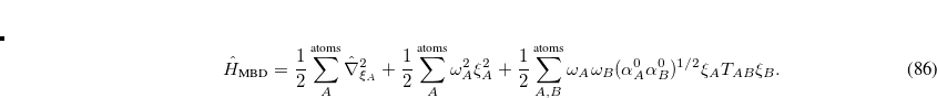 is the mass-weight displacement of oscillator from its center
 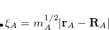 ,
,  is the characteristic frequency, and
  is the static polarizability.
  is the dipole potential between the oscillators and . The MBD Hamiltonian is obtained through coarse-graining of the long-range correlation (through the long-range dipole tensor
  ) and approximating the short-range polarizability via the adiabatic connection fluctuation-dissipation formula:
![\begin{equation} \label{eq:lrmbdcorr} E^{\mathrm{MBD}}_{c,\text {lr}}= -\sum _{n=2}^{\infty }\frac{(-1)^ n}{n}\int _0^\infty \frac{\mathrm{d} u}{2\pi } \sum _{AB}\mbox{tr}\Bigl [\bigl \langle (\mathbf{\alpha }_\mathrm {eff}\mathbf{T}_\mathrm {lr})^ n\bigl \rangle _{\! AB}(iu)\Bigr ] \; . \end{equation}](images/img-0499.png) |
(5.51) |
This approximation expresses the dynamic polarizability 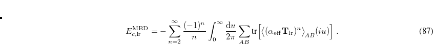 (of a given fragment) in terms of the polarizability of the corresponding QHO,
 |
(5.52) |
in which  is the charge,
  the mass, and the characteristic frequency of the oscillator. The integration in the frequency domain in Eq. eq:lrmbdcorr can be done analytically, leading to the so-called plasmon pole formula for the correlation energy,
 |
(5.53) |
in which  is the number of fragments,
 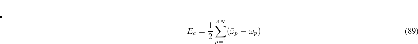 are the frequencies of the interacting (dipole-coupled) system, and
  are the frequencies of the non-interacting system (i.e., the collection of independent QHOs). The sum runs over all
  characteristic frequencies of the system.
A particular method within the MBD framework is defined by the models for the static polarizability ( ), the non-interacting characteristic frequencies (), and the damping function [
 ] used to define
  . In Q-Chem, the MBD method is implemented following the “MBD@rsSCS” approach, where “rsSCS” stands for range-separated self-consistent screening.[Ambrosetti et al.(2014)Ambrosetti, Reilly, DiStasio, Jr., and Tkatchenko] In this approach, is obtained in a two-step process:
The free-volume scaling approach is applied to the free-atom polarizabilities, using the Hirshfeld-partitioned molecular electron density. This is the same procedure used in the TS-vdW method described in Section 5.7.4.
The short-range atomic polarizabilities
 are obtained by applying a Dyson-like screening on only the short range part of the polarizabilities. The same range-separation will later be used to define .
The short-range atomic polarizabilities are summed up along one fragment coordinate to obtain the local effective dynamic polarizability, i.e.,  , and are then spherically averaged. The range-separation (damping) function used to construct and is the same as that in Eq. eq:fdamp_TS-vdW, except with
  instead of , and again for a given functional obtained by fitting to interaction energies for non-bonded complexes. The MBD energy is than calculated by diagonalizing the Hamiltonian Eq. eq:mbdhamil and using the plasmon-pole formula, Eq. eq:mbdplasmon.
The MBD-vdW approach greatly improves the accuracy of the interaction energies for S66[Řezáč et al.(2011)Řezáč, Riley, and Hobza] test set, even if a simple functional like PBE is used, with a mean absolute error of 0.3 kcal/mol and a maximum error of 1.3 kcal/mol, as compared to 2.3 kcal/mol (mean) and 7.2 kcal/mol (max) for plain PBE. In general, the MBD-vdW method is superior to pairwise a posteriori dispersion corrections.[Hermann et al.(2017)Hermann, DiStasio Jr., and Tkatchanko]
As mentioned above in the context of the TS-vdW method (Section 5.7.4), the FHI-aims or Quantum Espresso codes cannot perform exact unrestricted SCF calculations for the atoms and this leads to inconsistent free-atom volumes as compared to the sphericalized ones computed in Q-Chem, and thus inconsistent values for the vdW correction. Since the parameters of the TS-vdW and MBD-vdW models were fitted for use with FHI-aims and Quantum Espresso, results obtained using these codes are slightly closer to S66 benchmarks and thus scalar modifiers are available for the internally-computed Hirshfeld volume ratios in Q-Chem. For S66, the use of these modifiers leads to negligible differences between results obtained from all three codes.[Barton et al.()Barton, Lao, DiStasio, Jr., and Tkatchenko]
The MBD-vdW correction is requested by setting MBDVDM = TRUE in the $rem section. Other job control variables, including the aforementioned modifiers for the free-atom volume ratios, are the same as those for the TS-vdW method and are described in Section 5.7.4.
MBDVDW
Flag to switch on the MBD-vdW method
TYPE:
INTEGER
DEFAULT:
0
OPTIONS:
0
Do not calculate MBD.
1
Calculate the MBD-vdW contribution to the energy.
2
Calculate the MBD-vdW contribution to the energy and the gradient.
RECOMMENDATION:
NONE