5.5 DFT Numerical Quadrature

In practical DFT calculations, the forms of the approximate exchange-correlation functionals used are quite complicated, such that the required integrals involving the functionals generally cannot be evaluated analytically. Q-Chem evaluates these integrals through numerical quadrature directly applied to the exchange-correlation integrand. Several standard quadrature grids are available (“SG- $n$ ”, $n = 0, 1, 2, 3$ ), with a default value that is automatically set according to the complexity of the functional in question.

The quadrature approach in Q-Chem is generally similar to that found in many DFT programs. The multi-center XC integrals are first partitioned into “atomic” contributions using a nuclear weight function. Q-Chem uses the nuclear partitioning of Becke,[Becke(1988a)] though without the “atomic size adjustments” of Ref. Becke:1988a. The atomic integrals are then evaluated through standard one-center numerical techniques. Thus, the exchange-correlation energy is obtained as

$\begin{equation} \label{eq439} E_{\mathrm{XC}} =\sum _ A^{\rm atoms} \sum _{i\in A}^{\rm points} w_{Ai}^{} f(\mathbf{r}_{Ai}^{}) \; , \end{equation}$

(5.22)

where the function $f$ is the aforementioned XC integrand and the quantities 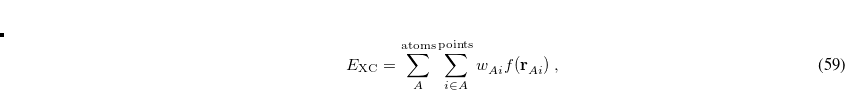$w_{Ai}$ are the quadrature weights. The sum over $i$ runs over grid points belonging to atom $A$ , which are located at positions $\mathbf{r}^{}_{Ai} = \mathbf{R}_ A^{} + \mathbf{r}_ i^{}$ , so this approach requires only the choice of a suitable one-center integration grid (to define the 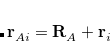$\mathbf{r}_ i^{}$ ), which is independent of nuclear configuration. These grids are implemented in Q-Chem in a way that ensures that the $E_{\rm XC}$ is rotationally-invariant, i.e., that is does not change when the molecule undergoes rigid rotation in space.[Johnson et al.(1994)Johnson, Gill, and Pople]

Quadrature grids are further separated into radial and angular parts. Within Q-Chem, the radial part is usually treated by the Euler-Maclaurin scheme proposed by Murray et al.,[Murray et al.(1993)Murray, Handy, and Laming] which maps the semi-infinite domain $[0,\infty )$ onto $[0,1)$ and applies the extended trapezoid rule to the transformed integrand. Alternatively, Gill and Chien proposed a radial scheme based on a Gaussian quadrature on the interval $[0,1]$ with a different weight function.[Chien and Gill(2003)] This “MultiExp" radial quadrature is exact for integrands that are a linear combination of a geometric sequence of exponential functions, and is therefore well suited to evaluating atomic integrals. However, the task of generating the MultiExp quadrature points becomes increasingly ill-conditioned as the number of radial points increases, so that a “double exponential" radial quadrature[Mitani(2011), Mitani and Yoshioka(2012)] is used for the largest standard grids in Q-Chem,[Mitani(2011), Mitani and Yoshioka(2012)] namely SG-2 and SG-3.[Dasgupta and Herbert(2017)] (See Section 5.5.2.)

5.5.1 Angular Grids

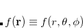
For a fixed value of the radial spherical-polar coordinate $r$ , a function $f(\mathbf{r}) \equiv f(r,\theta ,\phi )$ has an exact expansion in spherical harmonic functions,

$\begin{equation} f(r,\theta ,\phi ) = \sum _{\ell =0}^\infty \sum _{m=-\ell }^\ell c_{\ell m}^{} \mbox{Y}_{\ell m}(\theta ,\phi ) \; . \end{equation}$

(5.23)

Angular quadrature grids are designed to integrate 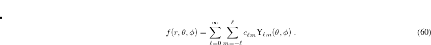$f(r,\theta ,\phi )$ for fixed $r$ , and are often characterized by their degree, meaning the maximum value of $\ell$ for which the quadrature is exact, as well as by their efficiency, meaning the number of spherical harmonics exactly integrated per degree of freedom in the formula. Q-Chem supports the following two types of angular grids.

Lebedev grids. These are specially-constructed grids for quadrature on the surface of a sphere,[Lebedev(1977), Lebedev(1975), Lebedev(1976), Lebedev and Laikov(1999)] based on the octahedral point group. Lebedev grids available in Q-Chem are listed in Table 5.2. These grids typically have near-unit efficiencies, with efficiencies exceeding unity in some cases. A Lebedev grid is selected by specifying the number of grid points (from Table 5.2) using the $rem keyword XC_GRID, as discussed below.

No. Points	Degree	No. Points	Degree	No. Points	Degree
	( $\bm@general \boldmath \m@ne \mv@bold \bm@command {\ell }_{\mathbf{max}}$ )		( $\bm@general \boldmath \m@ne \mv@bold \bm@command {\ell }_{\mathbf{max}}$ )		( $\bm@general \boldmath \m@ne \mv@bold \bm@command {\ell }_{\mathbf{max}}$ )
6	3	230	25	1730	71
14	5	266	27	2030	77
26	7	302	29	2354	83
38	9	350	31	2702	89
50	11	434	35	3074	95
74	13	590	41	3470	101
86	15	770	47	3890	107
110	17	974	53	4334	113
146	19	1202	59	4802	119
170	21	1454	65	5294	125
194	23

Table 5.2: Lebedev angular quadrature grids available in Q-Chem.

Gauss-Legendre grids. These are spherical direct-product grids in the two spherical-polar angles, $\theta$ and $\phi$ . Integration in over $\theta$ is performed using a Gaussian quadrature derived from the Legendre polynomials, while integration over $\phi$ is performed using equally-spaced points. A Gauss-Legendre grid is selected by specifying the total number of points, $2N^2$ , to be used for the integration, which specifies a grid consisting of $2N_{\phi }$ points in $\phi$ and $N_{\theta }$ in $\theta$ , for a degree of $2N-1$ . Gauss-Legendre grids exhibit efficiencies of only 2/3, and are thus lower in quality than Lebedev grids for the same number of grid points, but have the advantage that they are defined for arbitrary (and arbitrarily-large) numbers of grid points. This offers a mechanism to achieve arbitrary accuracy in the angular integration, if desired.

Combining these radial and angular schemes yields an intimidating selection of quadratures, so it is useful to standardize the grids. This is done for the convenience of the user, to facilitate comparisons in the literature, and also for developers wishing to compared detailed results between different software programs, because the total electronic energy is sensitive to the details of the grid, just as it is sensitive to details of the basis set. Standard quadrature grids are discussed next.

5.5.2 Standard Quadrature Grids

Four different “standard grids" are available in Q-Chem, designated SG- $n$ , for $n = 0, 1, 2$ , or 3; both quality and the computational cost of these grids increases with $n$ . These grids are constructed starting from a “parent” grid ( $N_ r,~ N_\Omega$ ) consisting of $N_ r$ radial spheres with $N_\Omega$ angular (Lebedev) grid points on each, then systematically pruning the number of angular points in regions where sophisticated angular quadrature is not necessary, such as near the nuclei where the charge density is nearly spherically symmetric and at long distance from the nuclei where it varies slowly. A large number of points is retained in the valence region where angular accuracy is critical. The SG- $n$ grids are summarized in Table 5.3. While many electronic structure programs use some kind of procedure to delete unnecessary grid points in the interest of computational efficiency, Q-Chem’s SG- $n$ grids are notable in that the complete grid specifications are available in the peer-reviewed literature,[Gill et al.(1993)Gill, Johnson, and Pople, Chien and Gill(2006), Dasgupta and Herbert(2017)] to facilitate reproduction of Q-Chem DFT calculations using other electronic structure programs. Just as computed energies may vary quite strongly with the choice of basis set, so too in DFT may they vary strongly with the choice of quadrature grid. In publications, users should always specify the grid that is used, and it is suggested to cite the appropriate literature reference from Table 5.3.

Pruned	Ref.	Parent Grid	No. Grid Points	Default Grid for
Grid		( $N_ r,N_\Omega$ )	(C atom) $^ a$	Which Functionals? $^ b$
SG-0	Chien:2006	(23, 170)	1,390 (36%)	None
SG-1	Gill:1993	(50, 194)	3,816 (39%)	LDA, most GGAs and hybrids
SG-2	Dasgupta:2017	(75, 302)	7,790 (34%)	Meta-GGAs; B95- and B97-based functionals
SG-3	Dasgupta:2017	(99, 590)	17,674 (30%)	Minnesota functionals
$^ a$ Number in parenthesis is the fraction of points retained from the parent grid
$^ b$ Reflects Q-Chem versions since v. 4.4.2

Table 5.3: Standard quadrature grids available in Q-Chem, along with the number of grid points for a carbon atom, showing the reduction in grid points due to pruning.

The SG-0 and SG-1 grids are designed for calculations on large molecules using GGA functionals. SG-1 affords integration errors on the order of $\sim$ 0.2 kcal/mol for medium-sized molecules and GGA functionals, including for demanding test cases such as reaction enthalpies for isomerizations. (Integration errors in total energies are no more than a few $\mu$ hartree, or $\sim$ 0.01 kcal/mol.) The SG-0 grid was derived in similar fashion, and affords a root-mean-square error in atomization energies of 72 $\mu$ hartree with respect to SG-1, while relative energies are reproduced well.[Chien and Gill(2006)] In either case, errors of this magnitude are typically considerably smaller than the intrinsic errors in GGA energies, and hence acceptable. As seen in Table 5.3, SG-1 retains $<40$ % of the grid points of its parent grid, which translates directly into cost savings.

Both SG-0 and SG-1 were optimized so that the integration error in the energy falls below a target threshold, but derivatives of the energy (including such properties as (hyper)polarizabilities[Castet and Champagne(2012)]) are often more sensitive to the quality of the integration grid. Special care is required, for example, when imaginary vibrational frequencies are encountered, as low-frequency (but real) vibrational frequencies can manifest as imaginary if the grid is sparse. If imaginary frequencies are found, or if there is some doubt about the frequencies reported by Q-Chem, the recommended procedure is to perform the geometry optimization and vibrational frequency calculations again using a higher-quality grid. (The optimization should converge quite quickly if the previously-optimized geometry is used as an initial guess.)

SG-1 was the default DFT integration grid for all density functionals for Q-Chem versions 3.2–4.4. Beginning with Q-Chem v. 4.4.2, however, the default grid is functional-dependent, as summarized in Table 5.3. This is a reflection of the fact that although SG-1 is adequate for energy calculations using most GGA and hybrid functionals (although care must be taken for some other properties, as discussed below), it is not adequate to integrate many functionals developed since $\sim$ 2005. These include meta-GGAs, which are more complicated due to their dependence on the kinetic energy density ( $\tau _\sigma$ in Eq. eq:tau) and/or the Laplacian of the density ( $\nabla ^2\rho _\sigma$ ). Functionals based on B97, along with the Minnesota suite of functionals,[Zhao and Truhlar(2008), Zhao and Truhlar(2011)] contain relatively complicated expressions for the exchange inhomogeneity factor, and are therefore also more sensitive to the quality of the integration grid.[Wheeler and Houk(2010), Mardirossian and Head-Gordon(2014), Dasgupta and Herbert(2017)] To integrate these modern density functionals, the SG-2 and SG-3 grids were developed,[Dasgupta and Herbert(2017)] which are pruned versions of the medium-quality (75, 302) and high-quality (99, 590) integration grids, respectively. Tests of properties known to be highly sensitive to the quality of the integration grid, such as vibrational frequencies, hyper-polarizabilities, and potential energy curves for non-bonded interactions, demonstrate that SG-2 is usually adequate for meta-GGAs and B97-based functionals, and in many cases is essentially converged with respect to an unpruned (250, 974) grid.[Dasgupta and Herbert(2017)] The Minnesota functionals are more sensitive to the grid, and while SG-3 is often adequate, it is not completely converged in the case of non-bonded interactions.[Dasgupta and Herbert(2017)]

Note: (1) SG-0 was re-optimized for Q-Chem v. 3.0, so results may differ slightly as compared to older versions of the program.
(2) The SG-2 and SG-3 grids use a double-exponential radial quadrature,[Dasgupta and Herbert(2017)] whereas a general grid (selected by setting XC_GRID = $XY$ , as described in Section 5.4) uses an Euler-MacLaurin radial quadrature. As such, absolute energies cannot be compared between, e.g., SG-2 and XC_GRID = 000075000302, even though SG-2 uses a pruned (75, 302) grid. However, energy differences should be quite similar between the two.

5.5.3 Consistency Check and Cutoffs

Whenever Q-Chem calculates numerical density functional integrals, the electron density itself is also integrated numerically as a test of the quality of the numerical quadrature. The extent to which this numerical result differs from the number of electrons is an indication of the accuracy of the other numerical integrals. A warning message is printed whenever the relative error in the numerical electron count reaches 0.01%, indicating that the numerical XC results may not be reliable. If the warning appears on the first SCF cycle it is probably not serious, because the initial-guess density matrix is sometimes not idempotent. This is the case with the SAD guess discussed in Section 4.4, and also with a density matrix that is taken from a previous geometry optimization cycle, and in such cases the problem will likely correct itself in subsequent SCF iterations. If the warning persists, however, then one should consider either using a finer grid or else selecting an alternative initial guess.

By default, Q-Chem will estimate the magnitude of various XC contributions on the grid and eliminate those determined to be numerically insignificant. Q-Chem uses specially-developed cutoff procedures which permits evaluation of the XC energy and potential in only ${\cal {O}}({N})$ work for large molecules. This is a significant improvement over the formal ${\cal {O}}({N^3})$ scaling of the XC cost, and is critical in enabling DFT calculations to be carried out on very large systems. In rare cases, however, the default cutoff scheme can be too aggressive, eliminating contributions that should be retained; this is almost always signaled by an inaccurate numerical density integral. An example of when this could occur is in calculating anions with multiple sets of diffuse functions in the basis. A remedy may be to increase the size of the quadrature grid.

5.5.4 Multi-resolution Exchange-Correlation (MRXC) Method

The multi-resolution exchange-correlation (MRXC) method is a new approach, courtesy of the Q-Chem development team,[Kong et al.(2006)Kong, Brown, and Fusti-Molnar, Russ et al.(2011)Russ, Chang, and Kong, Chang et al.(2011)Chang, Russ, and Kong] for accelerating computation of the exchange-correlation (XC) energy and matrix for any given density functional. As explained in Section 4.6.5, XC functionals are sufficiently complicated integration of them is usually performed by numerical quadrature. There are two basic types of quadrature. One is the atom-centered grid (ACG), a superposition of atomic quadrature described in Section 4.6.5. The ACG has high density of points near the nucleus to handle the compact core density and low density of points in the valence and non-bonding region where the electron density is smooth. The other type is even-spaced cubic grid (ESCG), which is typically used together with pseudopotentials and plane-wave basis functions where only the valence and non-bonded electron density is assumed smooth. In quantum chemistry, an ACG is more often used as it can handle accurately all-electron calculations of molecules. MRXC combines those two integration schemes seamlessly to achieve an optimal computational efficiency by placing the calculation of the smooth part of the density and XC matrix onto the ESCG. The computation associated with the smooth fraction of the electron density is the major bottleneck of the XC part of a DFT calculation and can be done at a much faster rate on the ESCG due to its low resolution. Fast Fourier transform and B-spline interpolation are employed for the accurate transformation between the two types of grids such that the final results remain the same as they would be on the ACG alone, yet a speedup of several times is achieved for the XC matrix. The smooth part of the calculation with MRXC can also be combined with FTC (see Section 4.6.5) to achieve a further gain in efficiency.

MRXC

Controls the use of MRXC.

TYPE:

INTEGER

DEFAULT:

0

OPTIONS:

0

Do not use MRXC

1

Use MRXC in the evaluation of the XC part

RECOMMENDATION:

MRXC is very efficient for medium and large molecules, especially when medium and large basis sets are used.

The following two keywords control the smoothness precision. The default value is carefully selected to maintain high accuracy.

MRXC_CLASS_THRESH_MULT

Controls the of smoothness precision

TYPE:

INTEGER

DEFAULT:

1

OPTIONS:

$im$

An integer

RECOMMENDATION:

A prefactor in the threshold for MRXC error control: $im\times 10^{-io}$

MRXC_CLASS_THRESH_ORDER

Controls the of smoothness precision

TYPE:

INTEGER

DEFAULT:

6

OPTIONS:

$io$

An integer

RECOMMENDATION:

The exponent in the threshold of the MRXC error control: $im\times 10^{-io}$

The next keyword controls the order of the B-spline interpolation:

LOCAL_INTERP_ORDER

Controls the order of the B-spline

TYPE:

INTEGER

DEFAULT:

6

OPTIONS:

$n$

An integer

RECOMMENDATION:

The default value is sufficiently accurate

5.5.5 Incremental DFT

Incremental DFT (IncDFT) uses the difference density and functional values to improve the performance of the DFT quadrature procedure by providing a better screening of negligible values. Using this option will yield improved efficiency at each successive iteration due to more effective screening.

INCDFT

Toggles the use of the IncDFT procedure for DFT energy calculations.

TYPE:

LOGICAL

DEFAULT:

TRUE

OPTIONS:

FALSE

Do not use IncDFT

TRUE

Use IncDFT

RECOMMENDATION:

Turning this option on can lead to faster SCF calculations, particularly towards the end of the SCF. Please note that for some systems use of this option may lead to convergence problems.

INCDFT_DENDIFF_THRESH

Sets the threshold for screening density matrix values in the IncDFT procedure.

TYPE:

INTEGER

DEFAULT:

SCF_CONVERGENCE + 3

OPTIONS:

$n$

Corresponding to a threshold of $10^{-n}$ .

RECOMMENDATION:

If the default value causes convergence problems, set this value higher to tighten the threshold.

INCDFT_GRIDDIFF_THRESH

Sets the threshold for screening functional values in the IncDFT procedure

TYPE:

INTEGER

DEFAULT:

SCF_CONVERGENCE + 3

OPTIONS:

$n$

Corresponding to a threshold of $10^{-n}$ .

RECOMMENDATION:

If the default value causes convergence problems, set this value higher to tighten the threshold.

INCDFT_DENDIFF_VARTHRESH

Sets the lower bound for the variable threshold for screening density matrix values in the IncDFT procedure. The threshold will begin at this value and then vary depending on the error in the current SCF iteration until the value specified by INCDFT_DENDIFF_THRESH is reached. This means this value must be set lower than INCDFT_DENDIFF_THRESH.

TYPE:

INTEGER

DEFAULT:

0

Variable threshold is not used.

OPTIONS:

$n$

Corresponding to a threshold of $10^{-n}$ .

RECOMMENDATION:

If the default value causes convergence problems, set this value higher to tighten accuracy. If this fails, set to 0 and use a static threshold.

INCDFT_GRIDDIFF_VARTHRESH

Sets the lower bound for the variable threshold for screening the functional values in the IncDFT procedure. The threshold will begin at this value and then vary depending on the error in the current SCF iteration until the value specified by INCDFT_GRIDDIFF_THRESH is reached. This means that this value must be set lower than INCDFT_GRIDDIFF_THRESH.

TYPE:

INTEGER

DEFAULT:

0

Variable threshold is not used.

OPTIONS:

$n$

Corresponding to a threshold of $10^{-n}$ .

RECOMMENDATION:

If the default value causes convergence problems, set this value higher to tighten accuracy. If this fails, set to 0 and use a static threshold.