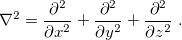
4.2 Theoretical Background

4.2.1 SCF and LCAO Approximations

The fundamental equation of non-relativistic quantum chemistry is the time-independent Schrödinger equation,

$\begin{equation} \label{eq400} \hat{H}({\rm {\bf R}},{\rm {\bf r}}) \; \Psi ({\rm {\bf R}},{\rm {\bf r}}) = E({\rm {\bf R}}) \; \Psi ({\rm {\bf R}},{\rm {\bf r}}) \; . \end{equation}$

(4.1)

In quantum chemistry, this equation is solved as a function of the electronic variables ( $\ensuremath{\mathbf{r}}$ ), for fixed values of the nuclear coordinates ( $\ensuremath{\mathbf{R}}$ ). The Hamiltonian operator in Eq. eq400, in atomic units, is

$\begin{equation} \label{eq:Hamiltonian} \hat{H}=-\frac{1}{2}\sum \limits _{i=1}^ N {\nabla _ i^2 } -\frac{1}{2}\sum \limits _{A=1}^ M {\frac{1}{M_ A }\nabla _ A^2 } -\sum \limits _{i=1}^ N {\sum \limits _{A=1}^ M {\frac{Z_ A }{r^{}_{iA} }} } +\sum \limits _{i=1}^ N {\sum \limits _{j>i}^ N {\frac{1}{r^{}_{ij} }} } +\sum \limits _{A=1}^ M {\sum \limits _{B>A}^ M {\frac{Z_ A Z_ B }{R_{AB} }} } \end{equation}$

(4.2)

where

$\begin{equation} \label{eq402} \nabla ^2 = \frac{\partial ^2}{\partial x^2}+\frac{\partial ^2}{\partial y^2}+\frac{\partial ^2}{\partial z^2} \; . \end{equation}$

(4.3)

In Eq. eq:Hamiltonian, $Z$ is the nuclear charge, $M_{A}$ is the ratio of the mass of nucleus $A$ to the mass of an electron, $R_{AB} = |\ensuremath{\mathbf{R}}_ A - \ensuremath{\mathbf{R}}_ B|$ is the distance between nuclei $A$ and $B$ , $r^{}_{ij} = |\ensuremath{\mathbf{r}}_{i} - \ensuremath{\mathbf{r}}_{j}|$ is the distance between the $i$ th and $j$ th electrons, $r^{}_{iA} = | \ensuremath{\mathbf{r}}_ i - \ensuremath{\mathbf{R}}_ A|$ is the distance between the $i$ th electron and the $A$ th nucleus, $M$ is the number of nuclei and $N$ is the number of electrons. The total energy $E$ is an eigenvalue of $\hat{H}$ , with a corresponding eigenfunction (wave function) $\Psi$ .

Separating the motions of the electrons from that of the nuclei, an idea originally due to Born and Oppenheimer [12], yields the electronic Hamiltonian operator:

$\begin{equation} \label{eq403} \hat{H}_{\mathrm{elec}} =-\frac{1}{2}\sum \limits _{i=1}^ N {\nabla _ i^2 } -\sum \limits _{i=1}^ N {\sum \limits _{A=1}^ M {\frac{Z_ A }{r^{}_{iA} }} } +\sum \limits _{i=1}^ N {\sum \limits _{j>i}^ N {\frac{1}{r^{}_{ij} }} } \end{equation}$

(4.4)

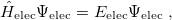
The solution of the corresponding electronic Schrödinger equation,

$\begin{equation} \label{eq404} \hat{H}_{\mathrm{elec}} \Psi _{\mathrm{elec}} =E_{\mathrm{elec}} \Psi _{\mathrm{elec}} \; , \end{equation}$

(4.5)

affords the total electronic energy, $E_{\mathrm{elec}}$ , and electronic wave function, $\Psi _{\mathrm{elec}}$ , which describes the distribution of the electrons for fixed nuclear positions. The total energy is obtained by simply adding the nuclear–nuclear repulsion energy [the fifth term in Eq. (4.2)] to the total electronic energy:

$\begin{equation} \label{eq405} E_{\mathrm{tot}} =E_{\mathrm{elec}} +E_{\mathrm{nuc}} \; . \end{equation}$

(4.6)

Solving the eigenvalue problem in Eq. (4.5) yields a set of eigenfunctions ( $\Psi _0$ , $\Psi _1$ , $\Psi _2 \ldots$ ) with corresponding eigenvalues $E_0 \le E_1 \le E_2 \le \ldots$ .

Our interest lies in determining the lowest eigenvalue and associated eigenfunction which correspond to the ground state energy and wave function of the molecule. However, solving Eq. (4.5) for other than the most trivial systems is extremely difficult and the best we can do in practice is to find approximate solutions.

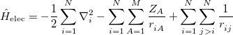
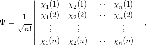
The first approximation used to solve Eq. eq404 is the independent-electron (mean-field) approximation, in which the wave function is approximated as an antisymmetrized product of one-electron functions, namely, the MOs. Each MO is determined by considering the electron as moving within an average field of all the other electrons. This affords the well-known Slater determinant wave function [13, 14]

$\begin{equation} \label{eq406} \Psi =\frac{1}{\sqrt {n!} }\left| {{\begin{array}{*{20}c} \chi ^{} _1(1) \hfill & \chi ^{}_2(1) \hfill & \cdots \hfill & \chi ^{}_ n (1) \hfill \\ \chi ^{} _1(2) \hfill & \chi ^{}_2(2) \hfill & \cdots \hfill & \chi ^{}_ n (2) \hfill \\ \vdots \hfill & \vdots \hfill & \hfill & \vdots \hfill \\ {\chi _1 (n)} \hfill & {\chi _2 (n)} \hfill & \cdots \hfill & {\chi _ n (n)} \hfill \\ \end{array} }} \right| \; , \end{equation}$

(4.7)

where $\chi _ i$ , a spin orbital, is the product of a molecular orbital $\psi _ i$ and a spin function ( $\alpha$ or $\beta$ ).

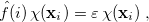
One obtains the optimum set of MOs by variationally minimizing the energy in what is called a “self-consistent field” or SCF approximation to the many-electron problem. The archetypal SCF method is the Hartree-Fock (HF) approximation, but these SCF methods also include KS-DFT (Section 4.4). All SCF methods lead to equations of the form

$\begin{equation} \label{eq407} \hat{f}(i) \, \chi (\ensuremath{\mathbf{x}}_ i )=\varepsilon \, \chi (\ensuremath{\mathbf{x}}_ i ) \; , \end{equation}$

(4.8)

where the Fock operator $\hat{f}(i)$ for the $i$ th electron is

$\begin{equation} \label{eq408} \hat{f}(i)=-\frac{1}{2}\nabla _ i^2 +\upsilon _{\rm eff}(i) \; . \end{equation}$

(4.9)

Here $\ensuremath{\mathbf{x}}_ i$ are spin and spatial coordinates of the $i$ th electron, the functions $\chi$ are spin orbitals and $\upsilon _{\rm eff}$ is the effective potential “seen” by the $i$ th electron, which depends on the spin orbitals of the other electrons. The nature of the effective potential $\upsilon _{\rm eff}$ depends on the SCF methodology, i.e., on the choice of density-functional approximation.

The second approximation usually introduced when solving Eq. eq404 is the introduction of an AO basis $\{ \phi _\mu \}$ linear combinations of which will then determine the MOs. There are many standardized, atom-centered Gaussian basis sets and details of these are discussed in Chapter 7.

After eliminating the spin components in Eq. (4.8) and introducing a finite basis,

$\begin{equation} \label{eq409} \psi _ i =\sum _\mu {c_{\mu i} \phi _\mu } \; , \end{equation}$

(4.10)

Eq. (4.8) reduces to the Roothaan-Hall matrix equation

$\begin{equation} \label{eq:Roothaan-Hall} \ensuremath{\mathbf{FC}} =\bm@general \boldmath \m@ne \mv@bold \bm@command {\varepsilon } \ensuremath{\mathbf{SC}} \; . \end{equation}$

(4.11)

Here, $\ensuremath{\mathbf{F}}$ is the Fock matrix, $\ensuremath{\mathbf{C}}$ is a square matrix of molecular orbital coefficients, $\ensuremath{\mathbf{S}}$ is the AO overlap matrix with elements

$\begin{equation} \label{eq411} S_{\mu \nu } =\int {\phi _\mu ({\rm {\bf r}})} \phi _\nu ({\rm {\bf r}})d{\rm {\bf r}} \end{equation}$

(4.12)

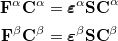
and $\bm@general \boldmath \m@ne \mv@bold \bm@command {\varepsilon }$ is a diagonal matrix containing the orbital energies. Generalizing to an unrestricted formalism by introducing separate spatial orbitals for $\alpha$ and $\beta$ spin in Eq. eq406 yields the Pople-Nesbet equations [15]

$\displaystyle \label{eq:Pople-Nesbet} \begin{aligned} \ensuremath{\mathbf{F}}^{\alpha } \ensuremath{\mathbf{C}}^{\alpha } & = \bm@general \boldmath \m@ne \mv@bold \bm@command {\varepsilon }^{\alpha } \ensuremath{\mathbf{SC}}^{\alpha } \\ \ensuremath{\mathbf{F}}^{\beta } \ensuremath{\mathbf{C}}^{\beta } & = \bm@general \boldmath \m@ne \mv@bold \bm@command {\varepsilon }^{\beta } \ensuremath{\mathbf{SC}}^{\beta } \end{aligned}$

(4.13)

In SCF methods, an initial guess is for the MOs is first determined, and from this, an average field seen by each electron can be calculated. A new set of MOs can be obtained by solving the Roothaan-Hall or Pople-Nesbet eigenvalue equations, resulting in the restricted or unrestricted finite-basis SCF approximation. This procedure is repeated until the new MOs differ negligibly from those of the previous iteration. The Hartree-Fock approximation for the effective potential in Eq. eq408 inherently neglects the instantaneous electron-electron correlations that are averaged out by the SCF procedure, and while the chemistry resulting from HF calculations often offers valuable qualitative insight, quantitative energetics are often poor. In principle, the DFT methodologies are able to capture all the correlation energy, i.e., the difference in energy between the HF energy and the true energy. In practice, the best-available density functionals perform well but not perfectly, and conventional post-HF approaches to calculating the correlation energy (see Chapter 5) are often required.

That said, because SCF methods often yield acceptably accurate chemical predictions at low- to moderate computational cost, self-consistent field methods are the cornerstone of most quantum-chemical programs and calculations. The formal costs of many SCF algorithms is ${\cal {O}}({N^4})$ , that is, they grow with the fourth power of system size, $N$ . This is slower than the growth of the cheapest conventional correlated methods, which scale as ${\cal {O}}({N^5})$ or worse, algorithmic advances available in Q-Chem can reduce the SCF cost to ${\cal {O}}({N})$ in favorable cases, an improvement that allows SCF methods to be applied to molecules previously considered beyond the scope of ab initio quantum chemistry.

In order to carry out an SCF calculation using Q-Chem, two $rem variables need to be set:

BASIS	to specify the basis set (see Chapter 7).
METHOD	SCF method: HF or a density functional (see Section 4.4).

Types of ground-state energy calculations currently available in Q-Chem are summarized in Table 4.1.

Calculation	$rem Variable JOBTYPE
Single point energy (default)	SINGLE_POINT or SP
Force (energy + gradient)	FORCE
Equilibrium structure search	OPTIMIZATION or OPT	(Ch. 9)
Transition structure search	TS	(Ch. 9)
Intrinsic reaction pathway	RPATH	(Sect. 9.5)
Potential energy scan	PES_SCAN	(Sect. 9.4)
Vibrational frequency calculation	FREQUENCY or FREQ	(Sect. 10.11 and 10.12)
NMR chemical shift	NMR	(Sect. 10.13
Indirect nuclear spin-spin coupling	ISSC	(Sect. 10.15
Ab initio molecular dynamics	AIMD	(Sect. 9.7
Ab initio path integrals	PIMD, PIMC	(Sect. 9.8)
BSSE (counterpoise) correction	BSSE	(Sect. 12.4.3)
Energy decomposition analysis	EDA	(Sect. 12.5)

Table 4.1: The type of calculation to be run by Q-Chem is controlled by the $rem variable JOBTYPE.

4.2.2 Hartree-Fock Theory

As with much of the theory underlying modern quantum chemistry, the HF approximation was developed shortly after publication of the Schrödinger equation, but remained a qualitative theory until the advent of the computer. Although the HF approximation tends to yield qualitative chemical accuracy, rather than quantitative information, and is generally inferior to many of the DFT approaches available, it remains as a useful tool in the quantum chemist’s toolkit. In particular, for organic chemistry, HF predictions of molecular structure are very useful.

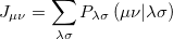
Consider once more the Roothaan-Hall equations, Eq. eq:Roothaan-Hall, or the Pople-Nesbet equations, Eq. eq:Pople-Nesbet, which can be traced back to Eq. eq407, in which the effective potential $\upsilon _{\rm eff}$ depends on the SCF methodology. In a restricted HF (RHF) formalism, the effective potential can be written as

$\begin{equation} \label{eq413} \upsilon _{\rm eff}=\sum _{a}^{N/2} \bigl [ {2\hat{J}_ a (1)-\hat{K}_ a (1)} \bigr ] -\sum _{A=1}^ M {\frac{Z_ A }{r^{}_{1A} }} \end{equation}$

(4.16)

where the Coulomb and exchange operators are defined as

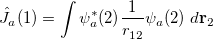$\begin{equation} \label{eq414} \Hat {J}_ a (1)=\int {\psi _ a^\ast (2)\frac{1}{r^{}_{12} }\psi _ a (2) \; d{\rm {\bf r}}_{ 2} } \end{equation}$

(4.17)

and

$\begin{equation} \label{eq415} \hat{K}_ a (1)\psi _ i (1)=\left[ {\int {\psi _ a^\ast (2)\frac{1}{r^{}_{12} }\psi _ i (2) \; d{\rm {\bf r}}_{ 2} } } \right]\psi _ a (1) \end{equation}$

(4.18)

respectively. By introducing an atomic orbital basis, we obtain Fock matrix elements

$\begin{equation} \label{eq416} F_{\mu \nu } =H_{\mu \nu }^{\mathrm{core}} +J_{\mu \nu } -K_{\mu \nu } \end{equation}$

(4.19)

where the core Hamiltonian matrix elements

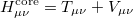$\begin{equation} \label{eq417} H_{\mu \nu }^{\mathrm{core}} =T_{\mu \nu } +V_{\mu \nu } \end{equation}$

(4.20)

consist of kinetic energy elements

$\begin{equation} \label{eq418} T_{\mu \nu } =\int {\phi _\mu ({\rm {\bf r}})\left( {-\frac{1}{2}\nabla ^2} \right)\phi _\nu ({\rm {\bf r}}) \; d{\rm {\bf r}}} \end{equation}$

(4.21)

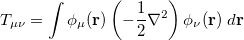
and nuclear attraction elements

$\begin{equation} \label{eq419} V_{\mu \nu } =\int {\phi _\mu ({\rm {\bf r}})\left( {-\sum \limits _ A {\frac{Z_ A }{\left| {{\rm {\bf R}}_{ A} -{\rm {\bf r}}} \right|}} } \right)\phi _\nu ({\rm {\bf r}}) \; d{\rm {\bf r}}} \end{equation}$

(4.22)

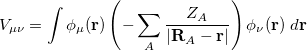
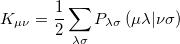
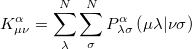
The Coulomb and exchange elements are given by

$\begin{equation} \label{eq420} J_{\mu \nu } =\sum \limits _{\lambda \sigma } {P_{\lambda \sigma } \left( {\mu \nu \vert \lambda \sigma } \right)} \end{equation}$

(4.23)

and

$\begin{equation} \label{eq421} K_{\mu \nu } =\frac{1}{2}\sum \limits _{\lambda \sigma } {P_{\lambda \sigma } \left( {\mu \lambda \vert \nu \sigma } \right)} \end{equation}$

(4.24)

respectively, where the density matrix elements are

$\begin{equation} \label{eq:P(mu,nu)} P_{\mu \nu } =2\sum \limits _{a=1}^{N/2} {C_{\mu a} C_{\nu a} } \end{equation}$

(4.25)

and the two electron integrals are

$\begin{equation} \label{eq423} \left( {\mu \nu \vert \lambda \sigma } \right)= \int \int {\phi _\mu ({\rm {\bf r}}_{ 1} )\phi _\nu ({\rm {\bf r}}_{ 1} ) \left( {\frac{1}{r^{}_{12} }} \right) \phi _\lambda ({\rm {\bf r}}_{ 2} )\phi _\sigma ({\rm {\bf r}}_{\rm {\bf 2}}) \; d{\rm {\bf r}}_{ 1} \; d{\rm {\bf r}}_{ 2} } \; . \end{equation}$

(4.26)

Note: The formation and utilization of two-electron integrals is a topic central to the overall performance of SCF methodologies. The performance of the SCF methods in new quantum chemistry software programs can be quickly estimated simply by considering the quality of their atomic orbital integrals packages. See Appendix B for details of Q-Chem’s AOInts package.

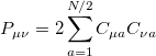
Substituting the matrix element in Eq. (4.19) back into the Roothaan-Hall equations, Eq. eq:Roothaan-Hall, and iterating until self-consistency is achieved will yield the RHF energy and wave function. Alternatively, one could have adopted the unrestricted form of the wave function by defining separate $\alpha$ and $\beta$ density matrices:

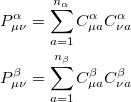$\displaystyle \label{eq424} \begin{aligned} P_{\mu \nu }^{\alpha } & = \sum \limits _{a=1}^{n_\alpha } {C_{\mu a}^\alpha C_{\nu a}^\alpha } \\ P_{\mu \nu }^{\beta } & = \sum \limits _{a=1}^{n_\beta } {C_{\mu a}^\beta C_{\nu a}^\beta } \end{aligned}$

(4.27)

The total electron density matrix $\ensuremath{\mathbf{P}} = \ensuremath{\mathbf{P}}^\alpha + \ensuremath{\mathbf{P}}^\beta$ . The unrestricted $\alpha$ Fock matrix,

$\begin{equation} \label{eq:F(mu,nu)} F_{\mu \nu }^\alpha =H_{\mu \nu }^{\mathrm{core}} +J_{\mu \nu } -K_{\mu \nu }^\alpha \; , \end{equation}$

(4.30)

differs from the restricted one only in the exchange contributions, where the $\alpha$ exchange matrix elements are given by

$\begin{equation} \label{eq426} K_{\mu \nu }^\alpha =\sum \limits _\lambda ^ N {\sum \limits _\sigma ^ N {P_{\lambda \sigma }^\alpha \left( {\mu \lambda \vert \nu \sigma } \right)} } \end{equation}$

(4.31)

4.2.3 Wave Function Stability Analysis

At convergence, the SCF energy will be at a stationary point with respect to changes in the MO coefficients. However, this stationary point is not guaranteed to be an energy minimum, and in cases where it is not, the wave function is said to be unstable. Even if the wave function is at a minimum, this minimum may be an artifact of the constraints placed on the form of the wave function. For example, an unrestricted calculation will usually give a lower energy than the corresponding restricted calculation, and this can give rise to a RHF $\rightarrow$ UHF instability.

To understand what instabilities can occur, it is useful to consider the most general form possible for the spin orbitals:

$\begin{equation} \label{eq427} \chi _ i ({\rm {\bf r}},\zeta )=\psi _ i^\alpha ({\rm {\bf r}})\alpha (\zeta )+\psi _ i^\beta ({\rm {\bf r}})\beta (\zeta ) \; . \end{equation}$

(4.32)

Here, $\psi _ i^\alpha$ and $\psi _ i^\beta$ are complex-valued functions of the Cartesian coordinates $\ensuremath{\mathbf{r}}$ , and $\alpha$ and $\beta$ are spin eigenfunctions of the spin-variable $\zeta$ . The first constraint that is almost universally applied is to assume the spin orbitals depend only on one or other of the spin-functions $\alpha$ or $\beta$ . Thus, the spin-functions take the form

$\begin{equation} \chi _ i(\ensuremath{\mathbf{r}},\zeta )=\psi _ i^\alpha (\ensuremath{\mathbf{r}})\alpha (\zeta ) \quad \mathrm{or} \quad \chi _ i(\ensuremath{\mathbf{r}},\zeta )=\psi _ i^\beta (\ensuremath{\mathbf{r}})\beta (\zeta ) \; . \end{equation}$

(4.33)

In addition, most SCF programs, including Q-Chem’s, deal only with real functions, and this places an additional constraint on the form of the wave function. If there exists a complex solution to the SCF equations that has a lower energy, the wave function exhibits a real $\rightarrow$ complex instability. The final constraint that is commonly placed on the spin-functions is that $\psi _ i^\alpha =\psi _ i^\beta$ , i.e., that the spatial parts of the spin-up and spin-down orbitals are the same. This gives the familiar restricted formalism and can lead to a RHF $\rightarrow$ UHF instability as mentioned above. Further details about the possible instabilities can be found in Ref. Seeger:1977.

Wave function instabilities can arise for several reasons, but frequently occur if

There exists a singlet diradical at a lower energy then the closed-shell singlet state.
There exists a triplet state at a lower energy than the lowest singlet state.
There are multiple solutions to the SCF equations, and the calculation has not found the lowest energy solution.

If a wave function exhibits an instability, the seriousness of it can be judged from the magnitude of the negative eigenvalues of the stability matrices. These matrices and eigenvalues are computed by Q-Chem’s Stability Analysis package, which was implemented by Dr Yihan Shao. The package is invoked by setting the STABILITY_ANALYSIS $rem variable equal to TRUE. In order to compute these stability matrices Q-Chem must first perform a CIS calculation. This will be performed automatically, and does not require any further input from the user. By default Q-Chem computes only the lowest eigenvalue of the stability matrix, which is usually sufficient to determine if there is a negative eigenvalue and thus an instability. To compute additional eigenvalues, set CIS_N_ROOTS $rem to a number larger than 1.

Q-Chem’s Stability Analysis package also seeks to correct internal instabilities (RHF $\rightarrow$ RHF or UHF $\rightarrow$ UHF). Then, if such an instability is detected, Q-Chem automatically performs a unitary transformation of the molecular orbitals following the directions of the lowest eigenvector, and writes a new set of MOs to disk. One can read in these MOs as an initial guess in a second SCF calculation (set the SCF_GUESS $rem variable to READ), it might also be desirable to set the SCF_ALGORITHM to GDM. In cases where the lowest-energy SCF solution breaks the molecular point-group symmetry, the SYM_IGNORE $rem should be set to TRUE.

Note: The stability analysis package can be used to analyze both DFT and HF wave functions.