9.7 Ab Initio Molecular Dynamics

Q-Chem can propagate classical molecular dynamics trajectories on the Born-Oppenheimer potential energy surface generated by a particular theoretical model chemistry (e.g., B3LYP/6-31G* or MP2/aug-cc-pVTZ). This procedure, in which the forces on the nuclei are evaluated on-the-fly, is known variously as “direct dynamics”, “ab initio molecular dynamics” (AIMD), or “Born-Oppenheimer molecular dynamics” (BOMD). In its most straightforward form, a BOMD calculation consists of an energy + gradient calculation at each molecular dynamics time step, and thus each time step is comparable in cost to one geometry optimization step. A BOMD calculation may be requested using any SCF energy + gradient method available in Q-Chem, including excited-state dynamics in cases where excited-state analytic gradients are available. As usual, Q-Chem will automatically evaluate derivatives by finite-difference if the analytic versions are not available for the requested method, but in AIMD applications this is very likely to be prohibitively expensive.

While the number of time steps required in most AIMD trajectories dictates that economical (typically SCF-based) underlying electronic structure methods are required, any method with available analytic gradients can reasonably be used for BOMD, including (within Q-Chem) HF, DFT, MP2, RI-MP2, CCSD, and CCSD(T). The RI-MP2 method, especially when combined with Fock matrix and $Z$ -vector extrapolation (as described below) is particularly effective as an alternative to DFT-based dynamics.

9.7.1 Overview and Basic Job Control

Initial Cartesian coordinates and velocities must be specified for the nuclei. Coordinates are specified in the $molecule section as usual, while velocities can be specified using a $velocity section with the form:

$velocity
$v_{x,1 }~ ~ ~ v_{y,1 }~ ~ ~ v_{z,1}$
$v_{x,2 }~ ~ ~ v_{y,2 }~ ~ ~ v_{z,2}$
$v_{x,N }~ ~ ~ v_{y,N }~ ~ ~ v_{z,N}$
$end

Here $v_{x,i}$ , $v_{y,i}$ , and $v_{z,i}$ are the $x$ , $y$ , and $z$ Cartesian velocities of the $i$ th nucleus, specified in atomic units (bohrs per atomic unit of time, where 1 a.u. of time is approximately 0.0242 fs). The $velocity section thus has the same form as the $molecule section, but without atomic symbols and without the line specifying charge and multiplicity. The atoms must be ordered in the same manner in both the $velocity and $molecule sections.

As an alternative to a $velocity section, initial nuclear velocities can be sampled from certain distributions (e.g., Maxwell-Boltzmann), using the AIMD_INIT_VELOC variable described below. AIMD_INIT_VELOC can also be set to QUASICLASSICAL, which triggers the use of quasi-classical trajectory molecular dynamics (see Section 9.7.5).

Although the Q-Chem output file dutifully records the progress of any ab initio molecular dynamics job, the most useful information is printed not to the main output file but rather to a directory called “AIMD” that is a subdirectory of the job’s scratch directory. (All ab initio molecular dynamics jobs should therefore use the –save option described in Section 2.7.) The AIMD directory consists of a set of files that record, in ASCII format, one line of information at each time step. Each file contains a few comment lines (indicated by “#”) that describe its contents and which we summarize in the list below.

Cost: Records the number of SCF cycles, the total CPU time, and the total memory use at each dynamics step.
EComponents: Records various components of the total energy (all in hartree).
Energy: Records the total energy and fluctuations therein.
MulMoments: If multipole moments are requested, they are printed here.
NucCarts: Records the nuclear Cartesian coordinates $x_{1}$ , $y_{1}$ , $z_{1}$ , $x_{2}$ , $y_{2}$ , $z_{2}$ , …, $x_{N}$ , $y_{N}$ , $z_{N}$ at each time step, in either bohrs or ngstroms.
NucForces: Records the Cartesian forces on the nuclei at each time step (same order as the coordinates, but given in atomic units).
NucVeloc: Records the Cartesian velocities of the nuclei at each time step (same order as the coordinates, but given in atomic units).
TandV: Records the kinetic and potential energy, as well as fluctuations in each.
View.xyz: Cartesian-formatted version of NucCarts for viewing trajectories in an external visualization program.

For ELMD jobs, there are other output files as well:

ChangeInF: Records the matrix norm and largest magnitude element of $\Delta \ensuremath{\mathbf{F}} = \ensuremath{\mathbf{F}}(t+\delta t) - \ensuremath{\mathbf{F}}(t)$ in the basis of Cholesky-orthogonalized AOs. The files ChangeInP, ChangeInL, and ChangeInZ provide analogous information for the density matrix $\ensuremath{\mathbf{P}}$ and the Cholesky orthogonalization matrices $\ensuremath{\mathbf{L}}$ and $\ensuremath{\mathbf{Z}}$ defined in [292].
DeltaNorm: Records the norm and largest magnitude element of the curvy-steps rotation angle matrix $\Delta$ defined in Ref. Herbert:2004. Matrix elements of $\Delta$ are the dynamical variables representing the electronic degrees of freedom. The output file DeltaDotNorm provides the same information for the electronic velocity matrix $d\Delta /{dt}$ .
ElecGradNorm: Records the norm and largest magnitude element of the electronic gradient matrix $\ensuremath{\mathbf{FP}} - \ensuremath{\mathbf{PF}}$ in the Cholesky basis.
dTfict: Records the instantaneous time derivative of the fictitious kinetic energy at each time step, in atomic units.

Ab initio molecular dynamics jobs are requested by specifying JOBTYPE = AIMD. Initial velocities must be specified either using a $velocity section or via the AIMD_INIT_VELOC keyword described below. In addition, the following $rem variables must be specified for any ab initio molecular dynamics job:

AIMD_METHOD

Selects an ab initio molecular dynamics algorithm.

TYPE:

STRING

DEFAULT:

BOMD

OPTIONS:

BOMD

Born-Oppenheimer molecular dynamics.

CURVY

Curvy-steps Extended Lagrangian molecular dynamics.

RECOMMENDATION:

BOMD yields exact classical molecular dynamics, provided that the energy is tolerably conserved. ELMD is an approximation to exact classical dynamics whose validity should be tested for the properties of interest.

TIME_STEP

Specifies the molecular dynamics time step, in atomic units (1 a.u. = 0.0242 fs).

TYPE:

INTEGER

DEFAULT:

None.

OPTIONS:

User-specified.

RECOMMENDATION:

Smaller time steps lead to better energy conservation; too large a time step may cause the job to fail entirely. Make the time step as large as possible, consistent with tolerable energy conservation.

AIMD_TIME_STEP_CONVERSION

Modifies the molecular dynamics time step to increase granularity.

TYPE:

INTEGER

DEFAULT:

1

OPTIONS:

$n$

The molecular dynamics time step is TIME_STEP/ $n$ a.u.

RECOMMENDATION:

None

AIMD_STEPS

Specifies the requested number of molecular dynamics steps.

TYPE:

INTEGER

DEFAULT:

None.

OPTIONS:

User-specified.

RECOMMENDATION:

None.

Ab initio molecular dynamics calculations can be quite expensive, and thus Q-Chem includes several algorithms designed to accelerate such calculations. At the self-consistent field (Hartree-Fock and DFT) level, BOMD calculations can be greatly accelerated by using information from previous time steps to construct a good initial guess for the new molecular orbitals or Fock matrix, thus hastening SCF convergence. A Fock matrix extrapolation procedure [567], based on a suggestion by Pulay and Fogarasi [568], is available for this purpose.

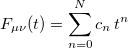
The Fock matrix elements $F_{\mu \nu }$ in the atomic orbital basis are oscillatory functions of the time $t$ , and Q-Chem’s extrapolation procedure fits these oscillations to a power series in $t$ :

$\begin{equation} F_{\mu \nu } (t)=\sum \limits _{n=0}^ N {c_ n \, } t^ n \end{equation}$

(9.14)

The $N+1$ extrapolation coefficients $c_ n$ are determined by a fit to a set of $M$ Fock matrices retained from previous time steps. Fock matrix extrapolation can significantly reduce the number of SCF iterations required at each time step, but for low-order extrapolations, or if SCF_CONVERGENCE is set too small, a systematic drift in the total energy may be observed. Benchmark calculations testing the limits of energy conservation can be found in Ref. Herbert:2005, and demonstrate that numerically exact classical dynamics (without energy drift) can be obtained at significantly reduced cost.

Fock matrix extrapolation is requested by specifying values for $N$ and $M$ , as in the form of the following two $rem variables:

FOCK_EXTRAP_ORDER

Specifies the polynomial order $N$ for Fock matrix extrapolation.

TYPE:

INTEGER

DEFAULT:

0

Do not perform Fock matrix extrapolation.

OPTIONS:

$N$

Extrapolate using an $N$ th-order polynomial ( $N > 0$ ).

RECOMMENDATION:

None

FOCK_EXTRAP_POINTS

Specifies the number $M$ of old Fock matrices that are retained for use in extrapolation.

TYPE:

INTEGER

DEFAULT:

0

Do not perform Fock matrix extrapolation.

OPTIONS:

$M$

Save $M$ Fock matrices for use in extrapolation $(M > N)$

RECOMMENDATION:

Higher-order extrapolations with more saved Fock matrices are faster and conserve energy better than low-order extrapolations, up to a point. In many cases, the scheme ( $N$ = 6, $M$ = 12), in conjunction with SCF_CONVERGENCE = 6, is found to provide about a 50% savings in computational cost while still conserving energy.

When nuclear forces are computed using underlying electronic structure methods with non-optimized orbitals (such as MP2), a set of response equations must be solved [569]. While these equations are linear, their dimensionality necessitates an iterative solution [570, 571], which, in practice, looks much like the SCF equations. Extrapolation is again useful here [293], and the syntax for $Z$ -vector (response) extrapolation is similar to Fock extrapolation.

Z_EXTRAP_ORDER

Specifies the polynomial order $N$ for Z-vector extrapolation.

TYPE:

INTEGER

DEFAULT:

0

Do not perform $Z$ -vector extrapolation.

OPTIONS:

$N$

Extrapolate using an $N$ th-order polynomial ( $N > 0$ ).

RECOMMENDATION:

None

Z_EXTRAP_POINTS

Specifies the number $M$ of old $Z$ -vectors that are retained for use in extrapolation.

TYPE:

INTEGER

DEFAULT:

0

Do not perform response equation extrapolation.

OPTIONS:

$M$

Save $M$ previous $Z$ -vectors for use in extrapolation $(M>N)$

RECOMMENDATION:

Using the default $Z$ -vector convergence settings, a $(M,N) = (4,2)$ extrapolation was shown to provide the greatest speedup. At this setting, a 2–3-fold reduction in iterations was demonstrated.

Assuming decent conservation, a BOMD calculation represents exact classical dynamics on the Born-Oppenheimer potential energy surface. In contrast, so-called extended Lagrangian molecular dynamics (ELMD) methods make an approximation to exact classical dynamics in order to expedite the calculations. ELMD methods—of which the most famous is Car–Parrinello molecular dynamics—introduce a fictitious dynamics for the electronic (orbital) degrees of freedom, which are then propagated alongside the nuclear degrees of freedom, rather than optimized at each time step as they are in a BOMD calculation. The fictitious electronic dynamics is controlled by a fictitious mass parameter $\mu$ , and the value of $\mu$ controls both the accuracy and the efficiency of the method. In the limit of small $\mu$ the nuclei and the orbitals propagate adiabatically, and ELMD mimics true classical dynamics. Larger values of $\mu$ slow down the electronic dynamics, allowing for larger time steps (and more computationally efficient dynamics), at the expense of an ever-greater approximation to true classical dynamics.

Q-Chem’s ELMD algorithm is based upon propagating the density matrix, expressed in a basis of atom-centered Gaussian orbitals, along shortest-distance paths (geodesics) of the manifold of allowed density matrices $\ensuremath{\mathbf{P}}$ . Idempotency of $\ensuremath{\mathbf{P}}$ is maintained at every time step, by construction, and thus our algorithm requires neither density matrix purification, nor iterative solution for Lagrange multipliers (to enforce orthogonality of the molecular orbitals). We call this procedure “curvy steps” ELMD [292], and in a sense it is a time-dependent implementation of the GDM algorithm (Section 4.6) for converging SCF single-point calculations.

The extent to which ELMD constitutes a significant approximation to BOMD continues to be debated. When assessing the accuracy of ELMD, the primary consideration is whether there exists a separation of time scales between nuclear oscillations, whose time scale $\tau _{\ensuremath{\mathrm{nuc}}}$ is set by the period of the fastest vibrational frequency, and electronic oscillations, whose time scale $\tau _{\ensuremath{\mathrm{elec}}}$ may be estimated according to [292]

$\begin{equation} \tau _{\ensuremath{\mathrm{elec}}} \geq \left(\frac{\mu }{\varepsilon ^{}_{\rm LUMO} - \varepsilon ^{}_{\rm HOMO}}\right)^{1/2} \end{equation}$

(9.15)

A conservative estimate, suggested in Ref. Herbert:2004, is that essentially exact classical dynamics is attained when $\tau _{\ensuremath{\mathrm{nuc}} }>$ 10 $\tau _{\ensuremath{\mathrm{elec}}}$ . In practice, we recommend careful benchmarking to insure that ELMD faithfully reproduces the BOMD observables of interest.

Due to the existence of a fast time scale $\tau _{\ensuremath{\mathrm{elec}}}$ , ELMD requires smaller time steps than BOMD. When BOMD is combined with Fock matrix extrapolation to accelerate convergence, it is no longer clear that ELMD methods are substantially more efficient, at least in Gaussian basis sets [567, 568].

The following $rem variables are required for ELMD jobs:

AIMD_FICT_MASS

Specifies the value of the fictitious electronic mass $\mu$ , in atomic units, where $\mu$ has dimensions of (energy) $\times$ (time) $^{2}$ .

TYPE:

INTEGER

DEFAULT:

None

OPTIONS:

User-specified

RECOMMENDATION:

Values in the range of 50–200 a.u. have been employed in test calculations; consult Ref. Herbert:2004 for examples and discussion.

9.7.2 Additional Job Control and Examples

AIMD_INIT_VELOC

Specifies the method for selecting initial nuclear velocities.

TYPE:

STRING

DEFAULT:

None

OPTIONS:

THERMAL

Random sampling of nuclear velocities from a Maxwell-Boltzmann

distribution. The user must specify the temperature in Kelvin via

the $rem variable AIMD_TEMP.

ZPE

Choose velocities in order to put zero-point vibrational energy into

each normal mode, with random signs. This option requires that a

frequency job to be run beforehand.

QUASICLASSICAL

Puts vibrational energy into each normal mode. In contrast to the

ZPE option, here the vibrational energies are sampled from a

Boltzmann distribution at the desired simulation temperature. This

also triggers several other options, as described below.

RECOMMENDATION:

This variable need only be specified in the event that velocities are not specified explicitly in a $velocity section.

AIMD_MOMENTS

Requests that multipole moments be output at each time step.

TYPE:

INTEGER

DEFAULT:

0

Do not output multipole moments.

OPTIONS:

$n$

Output the first $n$ multipole moments.

RECOMMENDATION:

None

AIMD_TEMP

Specifies a temperature (in Kelvin) for Maxwell-Boltzmann velocity sampling.

TYPE:

INTEGER

DEFAULT:

None

OPTIONS:

User-specified number of Kelvin.

RECOMMENDATION:

This variable is only useful in conjunction with AIMD_INIT_VELOC = THERMAL. Note that the simulations are run at constant energy, rather than constant temperature, so the mean nuclear kinetic energy will fluctuate in the course of the simulation.

DEUTERATE

Requests that all hydrogen atoms be replaces with deuterium.

TYPE:

LOGICAL

DEFAULT:

FALSE

Do not replace hydrogens.

OPTIONS:

TRUE

Replace hydrogens with deuterium.

RECOMMENDATION:

Replacing hydrogen atoms reduces the fastest vibrational frequencies by a factor of 1.4, which allow for a larger fictitious mass and time step in ELMD calculations. There is no reason to replace hydrogens in BOMD calculations.

Example 9.226 Simulating thermal fluctuations of the water dimer at 298 K.

$molecule
   0  1
   O   1.386977   0.011218   0.109098
   H   1.748442   0.720970  -0.431026
   H   1.741280  -0.793653  -0.281811
   O  -1.511955  -0.009629  -0.120521
   H  -0.558095   0.008225   0.047352
   H  -1.910308   0.077777   0.749067
$end

$rem
   JOBTYPE              aimd
   AIMD_METHOD          bomd
   METHOD               b3lyp
   BASIS                6-31g*
   TIME_STEP            20        (20 a.u. = 0.48 fs) 
   AIMD_STEPS           1000
   AIMD_INIT_VELOC      thermal
   AIMD_TEMP            298
   FOCK_EXTRAP_ORDER    6         request Fock matrix extrapolation
   FOCK_EXTRAP_POINTS   12 
$end

Example 9.227 Propagating $\rm F^-(H_2O)_4$ on its first excited-state potential energy surface, calculated at the CIS level.

$molecule
   -1   1
   O  -1.969902  -1.946636   0.714962
   H  -2.155172  -1.153127   1.216596
   H  -1.018352  -1.980061   0.682456
   O  -1.974264   0.720358   1.942703
   H  -2.153919   1.222737   1.148346
   H  -1.023012   0.684200   1.980531
   O  -1.962151   1.947857  -0.723321
   H  -2.143937   1.154349  -1.226245
   H  -1.010860   1.980414  -0.682958
   O  -1.957618  -0.718815  -1.950659
   H  -2.145835  -1.221322  -1.158379
   H  -1.005985  -0.682951  -1.978284
   F   1.431477   0.000499   0.010220
$end

$rem
   JOBTYPE           aimd
   AIMD_METHOD       bomd
   METHOD            hf
   BASIS             6-31+G*
   ECP               SRLC
   PURECART          1111
   CIS_N_ROOTS       3
   CIS_TRIPLETS      false
   CIS_STATE_DERIV   1         propagate on first excited state
   AIMD_INIT_VELOC   thermal
   AIMD_TEMP         150
   TIME_STEP         25
   AIMD_STEPS        827      (500 fs)
$end

Example 9.228 Simulating vibrations of the NaCl molecule using ELMD.

$molecule
   0  1
   Na   0.000000   0.000000  -1.742298 
   Cl   0.000000   0.000000   0.761479
$end

$rem
   JOBTYPE    freq
   METHOD     b3lyp
   ECP        sbkjc
$end

@@@

$molecule
   read
$end

$rem
   JOBTYPE           aimd
   METHOD            b3lyp
   ECP               sbkjc
   TIME_STEP         14
   AIMD_STEPS        500
   AIMD_METHOD       curvy
   AIMD_FICT_MASS    360
   AIMD_INIT_VELOC   zpe
$end

9.7.3 Thermostats: Sampling the NVT Ensemble

Implicit in the discussion above was an assumption of conservation of energy, which implies dynamics run in the microcanonical ( $NVE$ ) ensemble. Alternatively, the AIMD code in Q-Chem can sample the canonical ( $NVT$ ) ensemble with the aid of thermostats. These mimic the thermal effects of a surrounding temperature bath, and the time average of a trajectory (or trajectories) then affords thermodynamic averages at a chosen temperature. This option is appropriate in particular when multiple minima are thermally accessible. All sampled information is once again saved in the AIMD/ subdirectory of the $QCSCRATCH directory for the job. Thermodynamic averages and error analysis may be performed externally, using these data. Two commonly used thermostat options, both of which yield proper canonical distributions of the classical molecular motion, are implemented in Q-Chem and are described in more detail below. Constant-pressure barostats (for $NPT$ simulations) are not yet implemented.

As with any canonical sampling, the trajectory evolves at the mercy of barrier heights. Short trajectories will sample only within the local minimum of the initial conditions, which may be desired for sampling the properties of a given isomer, for example. Due to the energy fluctuations induced by the thermostat, the trajectory is neither guaranteed to stay within this potential energy well nor guaranteed to overcome barriers to neighboring minima, except in the infinite-sampling limit for the latter case, which is likely never reached in practice. Importantly, the user should note that the introduction of a thermostat destroys the validity of any real-time trajectory information; thermostatted trajectories should not be used to assess real-time dynamical observables, but only to compute thermodynamic averages.

9.7.3.1 Langevin Thermostat

A stochastic, white-noise Langevin thermostat (AIMD_THERMOSTAT = LANGEVIN) combines random “kicks” to the nuclear momenta with a dissipative, friction term. The balance of these two contributions mimics the exchange of energy with a surrounding heat bath. The resulting trajectory, in the long-time sampling limit, generates the correct canonical distribution. The implementation in Q-Chem follows the velocity Verlet formulation of Bussi and Parrinello,[572] which remains a valid propagator for all time steps and thermostat parameters. The thermostat is coupled to each degree of freedom in the simulated system. The MD integration time step (TIME_STEP) should be chosen in the same manner as in an NVE trajectory. The only user-controllable parameter for this thermostat, therefore, is the timescale over which the implied bath influences the trajectory. The AIMD_LANGEVIN_TIMESCALE keyword determines this parameter, in units of femtoseconds. For users who are more accustomed to thinking in terms of friction strength, this parameter is proportional to the inverse friction. A small value of the timescale parameter yields a “tight” thermostat, which strongly maintains the system at the chosen temperature but does not typically allow for rapid configurational flexibility. (Qualitatively, one may think of such simulations as sampling in molasses. This analogy, however, only applies to the thermodynamic sampling properties and does not suggest any electronic role of the solvent!) These small values are generally more appropriate for small systems, where the few degrees of freedom do not rapidly exchange energy and behave may behave in a non-ergodic fashion. Alternatively, large values of the time-scale parameter allow for more flexible configurational sampling, with the tradeoff of more (short-term) deviation from the desired average temperature. These larger values are more appropriate for larger systems since the inherent, microcanonical exchange of energy within the large number of degrees of freedom already tends toward canonical properties. (Think of this regime as sampling in a light, organic solvent.) Importantly, thermodynamic averages in the infinite-sampling limit are completely independent of this time-scale parameter. Instead, the time scale merely controls the efficiency with which the ensemble is explored. If maximum efficiency is desired, the user may externally compute lifetimes from the time correlation function of the desired observable and minimize the lifetime as a function of this timescale parameter. At the end of the trajectory, the average computed temperature is compared to the requested target temperature for validation purposes.

Example 9.229 Canonical ( $NVT$ ) sampling using AIMD with the Langevin thermostat

$comment
   Short example of using the Langevin thermostat
   for canonical (NVT) sampling
$end

$molecule
   0 1
   H
   O  1  1.0
   H  2  1.0  1  104.5
$end

$rem
   JOBTYPE                  aimd
   EXCHANGE                 hf
   BASIS                    sto-3g
   AIMD_TIME_STEP           20      !in au
   AIMD_STEPS               100       
   AIMD_THERMOSTAT          langevin
   AIMD_INIT_VELOC          thermal
   AIMD_TEMP                298     !in K - initial conditions AND thermostat
   AIMD_LANGEVIN_TIMESCALE  100     !in fs
$end

9.7.3.2 Nosé-Hoover Thermostat

An alternative thermostat approach is also available, namely, the Nosé-Hoover thermostat [573] (also known as a Nosé-Hoover “chain”), which mimics the role of a surrounding thermal bath by performing a microcanonical ( $NVE$ ) trajectory in an extended phase space. By allowing energy to be exchanged with a chain of fictitious particles that are coupled to the target system, $NVT$ sampling is properly obtained for those degrees of freedom that represent the real system. (Only the target system properties are saved in $QCSCRATCH/AIMD for subsequent analysis and visualization, not the fictitious Nosé-Hoover degrees of freedom.) The implementation in Q-Chem follows that of Martyna [573], which augments the original extended-Lagrangian approach of Nosé [574, 575] and Hoover [576], using a chain of auxiliary degrees of freedom to restore ergodicity in stiff systems and thus afford the correct $NVT$ ensemble. Unlike the Langevin thermostat, the collection of system and auxiliary chain particles can be propagated in a time-reversible fashion with no need for stochastic perturbations.

Rather than directly setting the masses and force constants of the auxiliary chain particles, the Q-Chem implementation focuses instead, on the time scale of the thermostat, as was the case for the Langevin thermostat described above. The time-scale parameter is controlled by the keyword NOSE_HOOVER_TIMESCALE, given in units of femtoseconds. The only other user-controllable parameter for this function is the length of the Nosé-Hoover chain, which is typically chosen to be 3–6 fictitious particles. Importantly, the version in Q-Chem is currently implemented as a single chain that is coupled to the system, as a whole. Comprehensive thermostatting in which every single degree of freedom is coupled to its own thermostat, which is sometimes used for particularly stiff systems, is not implemented and for such cases the Langevin thermostat is recommended instead. For large and/or fluxional systems, the single-chain Nosé-Hoover approach is appropriate.

Example 9.230 Canonical ( $NVT$ ) sampling using AIMD with the Nosé-Hoover chain thermostat

$molecule
   0 1
   H
   O 1 1.0 
   H 2 1.0 1 104.5
$end

$rem
   JOBTYPE                 aimd
   EXCHANGE                hf  
   BASIS                   sto-3g
   AIMD_TIME_STEP          20      !in au
   AIMD_STEPS              100
   AIMD_THERMOSTAT         nose_hoover
   AIMD_INIT_VELOC         thermal
   AIMD_TEMP               298     !in K - initial conditions AND thermostat
   NOSE_HOOVER_LENGTH      3       !chain length
   NOSE_HOOVER_TIMESCALE   100     !in fs
$end

AIMD_THERMOSTAT

Applies thermostatting to AIMD trajectories.

TYPE:

INTEGER

DEFAULT:

none

OPTIONS:

LANGEVIN

Stochastic, white-noise Langevin thermostat

NOSE_HOOVER

Time-reversible, Nosé-Hoovery chain thermostat

RECOMMENDATION:

Use either thermostat for sampling the canonical (NVT) ensemble.

AIMD_LANGEVIN_TIMESCALE

Sets the timescale (strength) of the Langevin thermostat

TYPE:

INTEGER

DEFAULT:

none

OPTIONS:

$n$

Thermostat timescale,asn $n$ fs

RECOMMENDATION:

Smaller values (roughly 100) equate to tighter thermostats but may inhibit rapid sampling. Larger values ( $\geq 1000$ ) allow for more rapid sampling but may take longer to reach thermal equilibrium.

NOSE_HOOVER_LENGTH

Sets the chain length for the Nosé-Hoover thermostat

TYPE:

INTEGER

DEFAULT:

none

OPTIONS:

$n$

Chain length of $n$ auxiliary variables

RECOMMENDATION:

Typically 3-6

NOSE_HOOVER_TIMESCALE

Sets the timescale (strength) of the Nosé-Hoover thermostat

TYPE:

INTEGER

DEFAULT:

none

OPTIONS:

$n$

Thermostat timescale, as $n$ fs

RECOMMENDATION:

Smaller values (roughly 100) equate to tighter thermostats but may inhibit rapid sampling. Larger values ( $\geq 1000$ ) allow for more rapid sampling but may take longer to reach thermal equilibrium.

9.7.4 Vibrational Spectra

The inherent nuclear motion of molecules is experimentally observed by the molecules’ response to impinging radiation. This response is typically calculated within the mechanical and electrical harmonic approximations (second derivative calculations) at critical-point structures. Spectra, including anharmonic effects, can also be obtained from dynamics simulations. These spectra are generated from dynamical response functions, which involve the Fourier transform of auto-correlation functions. Q-Chem can provide both the vibrational spectral density from the velocity auto-correlation function

$\begin{equation} D(\omega ) \propto \int _{-\infty }^{\infty } dt\ e^{-i\omega t} \langle \vec{v}(0)\bm@general \boldmath \m@ne \mv@bold \bm@command {\cdot }\vec{v}(t)\rangle \end{equation}$

(9.16)

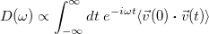
and infrared absorption intensity from the dipole auto-correlation function

$\begin{equation} I(\omega ) \propto \frac{\omega }{2\pi }\int _{-\infty }^{\infty } dt\ e^{-i\omega t} \langle \vec{\mu }(0)\bm@general \boldmath \m@ne \mv@bold \bm@command {\cdot }\vec{\mu }(t)\rangle \end{equation}$

(9.17)

These two features are activated by the AIMD_NUCL_VACF_POINTS and AIMD_NUCL_DACF_POINTS keywords, respectively, where values indicate the number of data points to include in the correlation function. Furthermore, the AIMD_NUCL_SAMPLE_RATE keyword controls the frequency at which these properties are sampled (entered as number of time steps). These spectra—generated at constant energy—should be averaged over a suitable distribution of initial conditions. The averaging indicated in the expressions above, for example, should be performed over a Boltzmann distribution of initial conditions.

Note that dipole auto-correlation functions can exhibit contaminating information if the molecule is allowed to rotate/translate. While the initial conditions in Q-Chem remove translation and rotation, numerical noise in the forces and propagation can lead to translation and rotation over time. The trans/rot correction in Q-Chem is activated by the PROJ_TRANSROT keyword.

AIMD_NUCL_VACF_POINTS

Number of time points to utilize in the velocity auto-correlation function for an AIMD trajectory

TYPE:

INTEGER

DEFAULT:

0

OPTIONS:

0

Do not compute velocity auto-correlation function.

$1\leq n \leq \mbox{{\small AIMD\_ STEPS}}$

Compute velocity auto-correlation function for last $n$

time steps of the trajectory.

RECOMMENDATION:

If the VACF is desired, set equal to AIMD_STEPS.

AIMD_NUCL_DACF_POINTS

Number of time points to utilize in the dipole auto-correlation function for an AIMD trajectory

TYPE:

INTEGER

DEFAULT:

0

OPTIONS:

0

Do not compute dipole auto-correlation function.

$1\leq n \leq \mbox{{\small AIMD\_ STEPS}}$

Compute dipole auto-correlation function for last $n$

timesteps of the trajectory.

RECOMMENDATION:

If the DACF is desired, set equal to AIMD_STEPS.

AIMD_NUCL_SAMPLE_RATE

The rate at which sampling is performed for the velocity and/or dipole auto-correlation function(s). Specified as a multiple of steps; i.e., sampling every step is 1.

TYPE:

INTEGER

DEFAULT:

None.

OPTIONS:

$1\leq n \leq \mbox{{\small AIMD\_ STEPS}}$

Update the velocity/dipole auto-correlation function

every $n$ steps.

RECOMMENDATION:

Since the velocity and dipole moment are routinely calculated for ab initio methods, this variable should almost always be set to 1 when the VACF/DACF are desired.

PROJ_TRANSROT

Removes translational and rotational drift during AIMD trajectories.

TYPE:

LOGICAL

DEFAULT:

FALSE

OPTIONS:

FALSE

Do not apply translation/rotation corrections.

TRUE

Apply translation/rotation corrections.

RECOMMENDATION:

When computing spectra (see AIMD_NUCL_DACF_POINTS, for example), this option can be utilized to remove artificial, contaminating peaks stemming from translational and/or rotational motion. Recommend setting to TRUE for all dynamics-based spectral simulations.

9.7.5 Quasi-Classical Molecular Dynamics

So-called “quasi-classical” trajectories [577, 578, 579] (QCT) put vibrational energy into each mode in the initial velocity setup step, which can improve on the results of purely classical simulations, for example in the calculation of photoelectron [580] or infrared spectra [581]. Improvements include better agreement of spectral linewidths with experiment at lower temperatures and better agreement of vibrational frequencies with anharmonic calculations.

The improvements at low temperatures can be understood by recalling that even at low temperature there is nuclear motion due to zero-point motion. This is included in the quasi-classical initial velocities, thus leading to finite peak widths even at low temperatures. In contrast to that the classical simulations yield zero peak width in the low temperature limit, because the thermal kinetic energy goes to zero as temperature decreases. Likewise, even at room temperature the quantum vibrational energy for high-frequency modes is often significantly larger than the classical kinetic energy. QCT-MD therefore typically samples regions of the potential energy surface that are higher in energy and thus more anharmonic than the low-energy regions accessible to classical simulations. These two effects can lead to improved peak widths as well as a more realistic sampling of the anharmonic parts of the potential energy surface. However, the QCT-MD method also has important limitations which are described below and that the user has to monitor for carefully.

In our QCT-MD implementation the initial vibrational quantum numbers are generated as random numbers sampled from a vibrational Boltzmann distribution at the desired simulation temperature. In order to enable reproducibility of the results, each trajectory (and thus its set of vibrational quantum numbers) is denoted by a unique number using the AIMD_QCT_WHICH_TRAJECTORY variable. In order to loop over different initial conditions, run trajectories with different choices for AIMD_QCT_WHICH_TRAJECTORY. It is also possible to assign initial velocities corresponding to an average over a certain number of trajectories by choosing a negative value. Further technical details of our QCT-MD implementation are described in detail in Appendix A of Ref. Lambrecht:2011.

AIMD_QCT_WHICH_TRAJECTORY

Picks a set of vibrational quantum numbers from a random distribution.

TYPE:

INTEGER

DEFAULT:

1

OPTIONS:

$n$

Picks the $n$ th set of random initial velocities.

$-n$

Uses an average over $n$ random initial velocities.

RECOMMENDATION:

Pick a positive number if you want the initial velocities to correspond to a particular set of vibrational occupation numbers and choose a different number for each of your trajectories. If initial velocities are desired that corresponds to an average over $n$ trajectories, pick a negative number.

Below is a simple example input for running a QCT-MD simulation of the vibrational spectrum of water. Most input variables are the same as for classical MD as described above. The use of quasi-classical initial conditions is triggered by setting the AIMD_INIT_VELOC variable to QUASICLASSICAL.

Example 9.231 Simulating the IR spectrum of water using QCT-MD.

$comment
   Don't forget to run a frequency calculation prior to this job.
$end

$molecule
   0  1
   O     0.000000    0.000000    0.520401
   H    -1.475015    0.000000   -0.557186
   H     1.475015    0.000000   -0.557186
$end


$rem
   JOBTYPE                     aimd
   INPUT_BOHR                  true
   METHOD                      hf
   BASIS                       3-21g
   SCF_CONVERGENCE             6
   TIME_STEP                   20  !  (in atomic units)
   AIMD_STEPS                  12500   6 ps total simulation time
   AIMD_TEMP                   12
   AIMD_PRINT                  2
   FOCK_EXTRAP_ORDER           6   ! Use a 6th-order extrapolation
   FOCK_EXTRAP_POINTS          12  ! of the previous 12 Fock matrices
   ! IR SPECTRAL SAMPLING
   AIMD_MOMENTS                1
   AIMD_NUCL_SAMPLE_RATE       5
   AIMD_NUCL_VACF_POINTS       1000
   ! QCT-SPECIFIC SETTINGS
   AIMD_INIT_VELOC            quasiclassical
   AIMD_QCT_WHICH_TRAJECTORY   1   ! Loop over several values to get
                                   ! the correct Boltzmann distribution.
$end

Other types of spectra can be calculated by calculating spectral properties along the trajectories. For example, we observed that photoelectron spectra can be approximated quite well by calculating vertical detachment energies (VDEs) along the trajectories and generating the spectrum as a histogram of the VDEs [580]. We have included several simple scripts in the $QC/aimdman/tools subdirectory that we hope the user will find helpful and that may serve as the basis for developing more sophisticated tools. For example, we include scripts that allow to perform calculations along a trajectory (md_calculate_along_trajectory) or to calculate vertical detachment energies along a trajectory (calculate_rel_energies).

Another application of the QCT code is to generate random geometries sampled from the vibrational wave function via a Monte Carlo algorithm. This is triggered by setting both the AIMD_QCT_INITPOS and AIMD_QCT_WHICH_TRAJECTORY variables to negative numbers, say $-m$ and $-n$ , and setting AIMD_STEPS to zero. This will generate $m$ random geometries sampled from the vibrational wave function corresponding to an average over $n$ trajectories at the user-specified simulation temperature.

AIMD_QCT_INITPOS

Chooses the initial geometry in a QCT-MD simulation.

TYPE:

INTEGER

DEFAULT:

0

OPTIONS:

$0$

Use the equilibrium geometry.

$n$

Picks a random geometry according to the harmonic vibrational wave function.

$-n$

Generates $n$ random geometries sampled from

the harmonic vibrational wave function.

RECOMMENDATION:

None.

For systems that are described well within the harmonic oscillator model and for properties that rely mainly on the ground-state dynamics, this simple MC approach may yield qualitatively correct spectra. In fact, one may argue that it is preferable over QCT-MD for describing vibrational effects at very low temperatures, since the geometries are sampled from a true quantum distribution (as opposed to classical and quasi-classical MD). We have included another script in the $QC/aimdman/tools directory to help with the calculation of vibrationally averaged properties (monte_geom).

Example 9.232 MC sampling of the vibrational wave function for HCl.

$comment
  Generates 1000 random geometries for HCl based on the harmonic vibrational 
  wave function at 1 Kelvin. The wave function is averaged over 1000
  sets of random vibrational quantum numbers (\ie{}, the ground state in
  this case due to the low temperature).
$end

$molecule
   0 1
   H    0.000000    0.000000   -1.216166
   Cl   0.000000    0.000000    0.071539
$end

$rem
   JOBTYPE                    aimd
   METHOD                     B3LYP
   BASIS                      6-311++G**
   SCF_CONVERGENCE            1
   SKIP_SCFMAN                1
   MAX_SCF_CYCLES             0
   XC_GRID                    1
   TIME_STEP                  20     (in atomic units)
   AIMD_STEPS                 0
   AIMD_INIT_VELOC            quasiclassical
   AIMD_QCT_VIBSEED           1
   AIMD_QCT_VELSEED           2
   AIMD_TEMP                  1     (in Kelvin)
   ! set aimd_qct_which_trajectory to the desired
   ! trajectory number
   AIMD_QCT_WHICH_TRAJECTORY  -1000
   AIMD_QCT_INITPOS           -1000
$end

It is also possible make some modes inactive, i.e., to put vibrational energy into a subset of modes (all other are set to zero). The list of active modes can be specified using the $qct_active_modes section. Furthermore, the vibrational quantum numbers for each mode can be specified explicitly using the $qct_vib_distribution input section. It is also possible to set the phases using $qct_vib_phase (allowed values are 1 and $-$ 1). Below is a simple sample input:

Example 9.233 User control over the QCT variables.

$comment
  Makes the 1st vibrational mode QCT-active; all other ones receive zero
  kinetic energy. We choose the vibrational ground state and a positive
  phase for the velocity. 
$end

...

$qct_active_modes
  1
$end

$qct_vib_distribution
  0
$end

$qct_vib_phase
  1
$end

...

Finally we turn to a brief description of the limitations of QCT-MD. Perhaps the most severe limitation stems from the so-called “kinetic energy spilling” problem [582], which means that there can be an artificial transfer of kinetic energy between modes. This can happen because the initial velocities are chosen according to quantum energy levels, which are usually much higher than those of the corresponding classical systems. Furthermore, the classical equations of motion also allow for the transfer of non-integer multiples of the zero-point energy between the modes, which leads to different selection rules for the transfer of kinetic energy. Typically, energy spills from high-energy into low-energy modes, leading to spurious “hot” dynamics. A second problem is that QCT-MD is actually based on classical Newtonian dynamics, which means that the probability distribution at low temperatures can be qualitatively wrong compared to the true quantum distribution [580].

Q-Chem implements a routine to monitor the kinetic energy within each normal mode along the trajectory and that is automatically switched on for quasi-classical simulations. It is thus possible to monitor for trajectories in which the kinetic energy in one or more modes becomes significantly larger than the initial energy. Such trajectories should be discarded. (Alternatively, see Ref. Czako:2010 for a different approach to the zero-point leakage problem.) Furthermore, this monitoring routine prints the squares of the (harmonic) vibrational wave function along the trajectory. This makes it possible to weight low-temperature results with the harmonic quantum distribution to alleviate the failure of classical dynamics for low temperatures.

9.7.6 Fewest-Switches Surface Hopping

As discussed in Section 9.6, optimization of minimum-energy crossing points (MECPs) along conical seams, followed by optimization of minimum-energy pathways that connect these MECPs to other points of interest on ground- and excited-state potential energy surfaces, affords an appealing one-dimensional picture of photochemical reactivity that is analogous to the “reactant $\rightarrow$ transition state $\rightarrow$ product” picture of ground-state chemistry. Just as the ground-state reaction is not obligated to proceed exactly through the transition-state geometry, however, an excited-state reaction need not proceed precisely through the MECP and the particulars of nuclear kinetic energy can lead to deviations. This is arguably more of an issue for excited-state reactions, where the existence of multiple conical intersections can easily lead to multiple potential reaction mechanisms. AIMD potentially offers a way to sample over the available mechanisms in order to deduce which ones are important in an automated way, but must be extended in the photochemical case to reactions that involve more than one Born-Oppenheimer potential energy surface.

The most widely-used trajectory-based method for non-adiabatic simulations is Tully’s “fewest-switches” surface-hopping (FSSH) algorithm [583, 584]. In this approach, classical trajectories are propagated on a single potential energy surface, but can undergo “hops” to a different potential surface in regions of near-degeneracy between surfaces. The probability of these stochastic hops is governed by the magnitude of the non-adiabatic coupling [Eq. eq:hJK]. Considering the ensemble average of a swarm of trajectories then provides information about, e.g., branching ratios for photochemical reactions.

The FSSH algorithm, based on the AIMD code, is available in Q-Chem for any electronic structure method where analytic derivative couplings are available, which at present means CIS, TDDFT, and their spin-flip analogues (see Section 9.6.1). The nuclear dynamics component of the simulation is specified just as in an AIMD calculation. Artificial decoherence can be added to the calculation at additional cost according to the augmented FSSH (AFSSH) method, [585, 586, 587] which enforces stochastic wave function collapse at a rate proportional to the difference in forces between the trajectory on the active surface and position moments propagated the other surfaces. At every time step, the component of the wave function on each active surface is printed to the output file. These amplitudes, as well as the position and momentum moments (if AFSSH is requested), is also printed to a text file called SurfaceHopper located in the $QC/AIMD sub-directory of the job’s scratch directory.

In order to request a FSSH calculation, only a few additional $rem variables must be added to those necessary for an excited-state AIMD simulation. At present, FSSH calculations can only be performed using Born-Oppenheimer molecular dynamics (BOMD) method. Furthermore, the optimized velocity Verlet (OVV) integration method is not supported for FSSH calculations.

FSSH_LOWESTSURFACE

Specifies the lowest-energy state considered in a surface hopping calculation.

TYPE:

INTEGER

DEFAULT:

None

OPTIONS:

$n$

Only states $n$ and above are considered in a FSSH calculation.

RECOMMENDATION:

None

FSSH_NSURFACES

Specifies the number of states considered in a surface hopping calculation.

TYPE:

INTEGER

DEFAULT:

None

OPTIONS:

$n$

$n$ states are considered in the surface hopping calculation.

RECOMMENDATION:

Any states which may come close in energy to the active surface should be included in the surface hopping calculation.

FSSH_INITIALSURFACE

Specifies the initial state in a surface hopping calculation.

TYPE:

INTEGER

DEFAULT:

None

OPTIONS:

$n$

An integer between FSSH_LOWESTSURFACE and FSSH_LOWESTSURFACE $+$ FSSH_NSURFACES $-1$ .

RECOMMENDATION:

None

AFSSH

Adds decoherence approximation to surface hopping calculation.

TYPE:

INTEGER

DEFAULT:

0

OPTIONS:

0

Traditional surface hopping, no decoherence.

1

Use augmented fewest-switches surface hopping (AFSSH).

RECOMMENDATION:

AFSSH will increase the cost of the calculation, but may improve accuracy for some systems. See Refs. Subotnik:2011a,Subotnik:2011b,Landry:2012 for more detail.

AIMD_SHORT_TIME_STEP

Specifies a shorter electronic time step for FSSH calculations.

TYPE:

INTEGER

DEFAULT:

TIME_STEP

OPTIONS:

$n$

Specify an electronic time step duration of $n$ /AIMD_TIME_STEP_CONVERSION

a.u. If $n$ is less than the nuclear time step variable TIME_STEP, the

electronic wave function will be integrated multiple times per nuclear time step,

using a linear interpolation of nuclear quantities such as the energy gradient and

derivative coupling. Note that $n$ must divide TIME_STEP evenly.

RECOMMENDATION:

Make AIMD_SHORT_TIME_STEP as large as possible while keeping the trace of the density matrix close to unity during long simulations. Note that while specifying an appropriate duration for the electronic time step is essential for maintaining accurate wave function time evolution, the electronic-only time steps employ linear interpolation to estimate important quantities. Consequently, a short electronic time step is not a substitute for a reasonable nuclear time step.

FSSH_CONTINUE

Restart a FSSH calculation from a previous run, using the file 396.0. When this is enabled, the initial conditions of the surface hopping calculation will be set, including the correct wave function amplitudes, initial surface, and position/momentum moments (if AFSSH) from the final step of some prior calculation.

TYPE:

INTEGER

DEFAULT:

0

OPTIONS:

$0$

Start fresh calculation.

$1$

Restart from previous run.

RECOMMENDATION:

None

Example 9.234 FSSH simulation. Note that analytic derivative couplings must be requested via CALC_NAC, but it is unnecessary to include a $derivative_coupling section. The same is true for SET_STATE_DERIV, which will be set to the initial active surface automatically. Finally, one must be careful to choose a small enough time step for systems that have energetic access to a region of large derivative coupling, hence the choice for AIMD_TIME_STEP_CONVERSION and TIME_STEP.

$molecule
   0 1
   C   -1.620294    0.348677   -0.008838
   C   -0.399206   -0.437493   -0.012535
   C   -0.105193   -1.296810   -1.081340
   H   -0.789110   -1.374693   -1.905080
   C    1.069016   -2.045054   -1.072304
   H    1.292495   -2.701157   -1.889686
   C    1.956240   -1.940324    0.002842
   H    2.859680   -2.517019    0.008420
   C    1.666259   -1.084065    1.071007
   H    2.348104   -1.005765    1.894140
   C    0.495542   -0.335701    1.065497
   H    0.253287    0.325843    1.871866
   O   -1.931045    1.124872    0.911738
   H   -2.269528    0.227813   -0.865645
$end

$rem
   JOBTYPE                    aimd
   EXCHANGE                   hf
   BASIS                      3-21g
   CIS_N_ROOTS                2
   SYMMETRY                   off
   SYM_IGNORE                 true
   CIS_SINGLETS               false
   CIS_TRIPLETS               true
   PROJ_TRANSROT              true
   FSSH_LOWESTSURFACE         1
   FSSH_NSURFACES             2 ! hop between T1 and T2
   FSSH_INITIALSURFACE        1 ! start on T1
   AFSSH                      0 ! no decoherence
   CALC_NAC                   true
   AIMD_STEPS                 500
   TIME_STEP                  14
   AIMD_SHORT_TIME_STEP       2
   AIMD_TIME_STEP_CONVERSION  1 ! Do not alter time_step duration
   AIMD_PRINT                 1
   AIMD_INIT_VELOC            thermal
   AIMD_TEMP                  300 # K
   AIMD_THERMOSTAT            4 # Langevin
   AIMD_INTEGRATION           vverlet
   FOCK_EXTRAP_ORDER          6
   FOCK_EXTRAP_POINTS         12
$end

BOMD	Born-Oppenheimer molecular dynamics.
CURVY	Curvy-steps Extended Lagrangian molecular dynamics.

THERMAL	Random sampling of nuclear velocities from a Maxwell-Boltzmann
	distribution. The user must specify the temperature in Kelvin via
	the $rem variable AIMD_TEMP.
ZPE	Choose velocities in order to put zero-point vibrational energy into
	each normal mode, with random signs. This option requires that a
	frequency job to be run beforehand.
QUASICLASSICAL	Puts vibrational energy into each normal mode. In contrast to the
	ZPE option, here the vibrational energies are sampled from a
	Boltzmann distribution at the desired simulation temperature. This
	also triggers several other options, as described below.

LANGEVIN	Stochastic, white-noise Langevin thermostat
NOSE_HOOVER	Time-reversible, Nosé-Hoovery chain thermostat

0	Do not compute velocity auto-correlation function.
$1\leq n \leq \mbox{{\small AIMD\_ STEPS}}$	Compute velocity auto-correlation function for last $n$
	time steps of the trajectory.

0	Do not compute dipole auto-correlation function.
$1\leq n \leq \mbox{{\small AIMD\_ STEPS}}$	Compute dipole auto-correlation function for last $n$
	timesteps of the trajectory.

$1\leq n \leq \mbox{{\small AIMD\_ STEPS}}$	Update the velocity/dipole auto-correlation function
	every $n$ steps.

FALSE	Do not apply translation/rotation corrections.
TRUE	Apply translation/rotation corrections.

0	Traditional surface hopping, no decoherence.
1	Use augmented fewest-switches surface hopping (AFSSH).

$n$	Specify an electronic time step duration of $n$ /AIMD_TIME_STEP_CONVERSION
	a.u. If $n$ is less than the nuclear time step variable TIME_STEP, the
	electronic wave function will be integrated multiple times per nuclear time step,
	using a linear interpolation of nuclear quantities such as the energy gradient and
	derivative coupling. Note that $n$ must divide TIME_STEP evenly.