10.12 Anharmonic Vibrational Frequencies
Computing vibrational spectra beyond the harmonic approximation has become an active area of research owing to the improved efficiency of computer techniques [662, 663, 664, 665]. To calculate the exact vibrational spectrum within Born-Oppenheimer approximation, one has to solve the nuclear Schrödinger equation completely using numerical integration techniques, and consider the full configuration interaction of quanta in the vibrational states. This has only been carried out on di- or triatomic system [666, 667]. The difficulty of this numerical integration arises because solving exact the nuclear Schrödinger equation requires a complete electronic basis set, consideration of all the nuclear vibrational configuration states, and a complete potential energy surface (PES). Simplification of the Nuclear Vibration Theory (NVT) and PES are the doorways to accelerating the anharmonic correction calculations. There are five aspects to simplifying the problem:
Expand the potential energy surface using a Taylor series and examine the contribution from higher derivatives. Small contributions can be eliminated, which allows for the efficient calculation of the Hamiltonian.
Investigate the effect on the number of configurations employed in a variational calculation.
Avoid using variational theory (due to its expensive computational cost) by using other approximations, for example, perturbation theory.
Obtain the PES indirectly by applying a self-consistent field procedure.
Apply an anharmonic wave function which is more appropriate for describing the distribution of nuclear probability on an anharmonic potential energy surface.
To incorporate these simplifications, new formulae combining information from the Hessian, gradient and energy are used as a default procedure to calculate the cubic and quartic force field of a given potential energy surface.
Here, we also briefly describe various NVT methods. In the early stage of solving the nuclear Schrödinger equation (in the 1930s), second-order Vibrational Perturbation Theory (VPT2) was developed [668, 669, 670, 671, 665]. However, problems occur when resonances exist in the spectrum. This becomes more problematic for larger molecules due to the greater chance of accidental degeneracies occurring. To avoid this problem, one can do a direct integration of the secular matrix using Vibrational Configuration Interaction (VCI) theory [672]. It is the most accurate method and also the least favored due to its computational expense. In Q-Chem 3.0, we introduce a new approach to treating the wave function, transition-optimized shifted Hermite (TOSH) theory [673], which uses first-order perturbation theory, which avoids the degeneracy problems of VPT2, but which incorporates anharmonic effects into the wave function, thus increasing the accuracy of the predicted anharmonic energies.
10.12.1 Vibration Configuration Interaction Theory
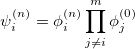
To solve the nuclear vibrational Schrödinger equation, one can only use direct integration procedures for diatomic molecules [666, 667]. For larger systems, a truncated version of full configuration interaction is considered to be the most accurate approach. When one applies the variational principle to the vibrational problem, a basis function for the nuclear wave function of the  th excited state of mode
  is
is
 |
(10.43) |
where the  represents the harmonic oscillator eigenfunctions for normal mode
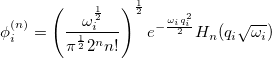
  . This can be expressed in terms of Hermite polynomials:
 |
(10.44) |
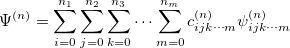
With the basis function defined in Eq. (10.43), the th wave function can be described as a linear combination of the Hermite polynomials:
 |
(10.45) |
where  is the number of quanta in the th mode. We propose the notation VCI() where is the total number of quanta, i.e.:
 |
(10.46) |
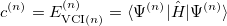
To determine this expansion coefficient  , we integrate the
  , as in Eq. (4.1), with
  to get the eigenvalues
 |
(10.47) |
This gives us frequencies that are corrected for anharmonicity to quanta accuracy for a  -mode molecule. The size of the secular matrix on the right hand of Eq. (10.47) is
  , and the storage of this matrix can easily surpass the memory limit of a computer. Although this method is highly accurate, we need to seek for other approximations for computing large molecules.
10.12.2 Vibrational Perturbation Theory
Vibrational perturbation theory has been historically popular for calculating molecular spectroscopy. Nevertheless, it is notorious for the inability of dealing with resonance cases. In addition, the non-standard formulas for various symmetries of molecules forces the users to modify inputs on a case-by-case basis [674, 675, 676], which narrows the accessibility of this method. VPT applies perturbation treatments on the same Hamiltonian as in Eq. (4.1), but divides it into an unperturbed part,  ,
,
 |
(10.48) |
and a perturbed part,  :
:
 |
(10.49) |
One can then apply second-order perturbation theory to get the th excited state energy:
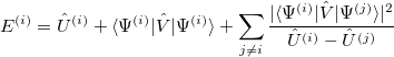 |
(10.50) |
The denominator in Eq. (10.50) can be zero either because of symmetry or accidental degeneracy. Various solutions, which depend on the type of degeneracy that occurs, have been developed which ignore the zero-denominator elements from the Hamiltonian [677, 674, 675, 676]. An alternative solution has been proposed by Barone [665] which can be applied to all molecules by changing the masses of one or more nuclei in degenerate cases. The disadvantage of this method is that it will break the degeneracy which results in fundamental frequencies no longer retaining their correct symmetry. He proposed
 |
(10.51) |
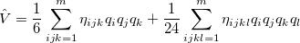
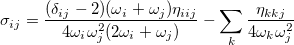
where, if rotational coupling is ignored, the anharmonic constants  are given by
![\begin{equation} x_{ij} = \frac{1}{4\omega _ i\omega _ j} \left( \eta _{iijj} - \sum _ k^ m \frac{\eta _{iik}\eta _{jjk}}{\omega _ k^2} + \sum _ k^ m \frac{2(\omega _ i^2+\omega _ j^2-\omega _ k^2)\eta _{ijk}^2}{ \left[(\omega _ i+\omega _ j)^2-\omega _ k^2\right] \left[(\omega _ i-\omega _ j)^2-\omega _ k^2\right]}\right) \end{equation}](images/img-1600.png) |
(10.52) |
10.12.3 Transition-Optimized Shifted Hermite Theory
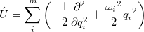
So far, every aspect of solving the nuclear wave equation has been considered, except the wave function. Since Schrödinger proposed his equation, the nuclear wave function has traditionally be expressed in terms of Hermite functions, which are designed for the harmonic oscillator case. Recently [673], a modified representation has been presented. To demonstrate how this approximation works, we start with a simple example. For a diatomic molecule, the Hamiltonian with up to quartic derivatives can be written as
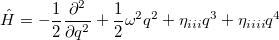 |
(10.53) |
and the wave function is expressed as in Eq. (10.44). Now, if we shift the center of the wave function by  , which is equivalent to a translation of the normal coordinate
  , the shape will still remain the same, but the anharmonic correction can now be incorporated into the wave function. For a ground vibrational state, the wave function is written as
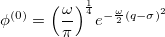 |
(10.54) |
Similarly, for the first excited vibrational state, we have
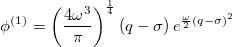 |
(10.55) |
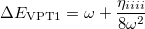
Therefore, the energy difference between the first vibrational excited state and the ground state is
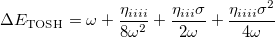 |
(10.56) |
This is the fundamental vibrational frequency from first-order perturbation theory.
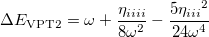
Meanwhile, We know from the first-order perturbation theory with an ordinary wave function within a QFF PES, the energy is
 |
(10.57) |
The differences between these two wave functions are the two extra terms arising from the shift in Eq. (10.56). To determine the shift, we compare the energy with that from second-order perturbation theory:
 |
(10.58) |
Since is a very small quantity compared with the other variables, we ignore the contribution of  and compare
  with
with  , which yields an initial guess for :
 |
(10.59) |
Because the only difference between this approach and the ordinary wave function is the shift in the normal coordinate, we call it “transition-optimized shifted Hermite” (TOSH) functions [673]. This approximation gives second-order accuracy at only first-order cost.
For polyatomic molecules, we consider Eq. (10.56), and propose that the energy of the th mode be expressed as:
 |
(10.60) |
Following the same approach as for the diatomic case, by comparing this with the energy from second-order perturbation theory, we obtain the shift as
 |
(10.61) |
10.12.4 Job Control
The following $rem variables can be used to control the calculation of anharmonic frequencies.
ANHAR
Performing various nuclear vibrational theory (TOSH, VPT2, VCI) calculations to obtain vibrational anharmonic frequencies.
TYPE:
LOGICAL
DEFAULT:
FALSE
OPTIONS:
TRUE
Carry out the anharmonic frequency calculation.
FALSE
Do harmonic frequency calculation.
RECOMMENDATION:
Since this calculation involves the third and fourth derivatives at the minimum of the potential energy surface, it is recommended that the GEOM_OPT_TOL_DISPLACEMENT, GEOM_OPT_TOL_GRADIENT and GEOM_OPT_TOL_ENERGY tolerances are set tighter. Note that VPT2 calculations may fail if the system involves accidental degenerate resonances. See the VCI $rem variable for more details about increasing the accuracy of anharmonic calculations.
VCI
Specifies the number of quanta involved in the VCI calculation.
TYPE:
INTEGER
DEFAULT:
0
OPTIONS:
User-defined. Maximum value is 10.
RECOMMENDATION:
The availability depends on the memory of the machine. Memory allocation for VCI calculation is the square of
with double precision. For example, a machine with 1.5 Gb memory and for molecules with fewer than 4 atoms, VCI(10) can be carried out, for molecule containing fewer than 5 atoms, VCI(6) can be carried out, for molecule containing fewer than 6 atoms, VCI(5) can be carried out. For molecules containing fewer than 50 atoms, VCI(2) is available. VCI(1) and VCI(3) usually overestimated the true energy while VCI(4) usually gives an answer close to the converged energy.
FDIFF_DER
Controls what types of information are used to compute higher derivatives. The default uses a combination of energy, gradient and Hessian information, which makes the force field calculation faster.
TYPE:
INTEGER
DEFAULT:
3
for jobs where analytical 2nd derivatives are available.
0
for jobs with ECP.
OPTIONS:
0
Use energy information only.
1
Use gradient information only.
2
Use Hessian information only.
3
Use energy, gradient, and Hessian information.
RECOMMENDATION:
When the molecule is larger than benzene with small basis set, FDIFF_DER=2 may be faster. Note that FDIFF_DER will be set lower if analytic derivatives of the requested order are not available. Please refers to IDERIV.
MODE_COUPLING
Number of modes coupling in the third and fourth derivatives calculation.
TYPE:
INTEGER
DEFAULT:
2
for two modes coupling.
OPTIONS:
for
RECOMMENDATION:
Use the default.
IGNORE_LOW_FREQ
Low frequencies that should be treated as rotation can be ignored during
anharmonic correction calculation.
TYPE:
INTEGER
DEFAULT:
300
Corresponding to 300 cm
.
OPTIONS:
Any mode with harmonic frequency less than
RECOMMENDATION:
Use the default.
FDIFF_STEPSIZE_QFF
Displacement used for calculating third and fourth derivatives by finite difference.
TYPE:
INTEGER
DEFAULT:
5291
Corresponding to 0.1 bohr. For calculating third and fourth derivatives.
OPTIONS:
Use a step size of
.
RECOMMENDATION:
Use the default, unless the potential surface is very flat, in which case a larger value should be used.
Example 10.252 A four-quanta anharmonic frequency calculation on formaldehyde at the EDF2/6-31G* optimized ground state geometry, which is obtained in the first part of the job. It is necessary to carry out the harmonic frequency first and this will print out an approximate time for the subsequent anharmonic frequency calculation. If a FREQ job has already been performed, the anharmonic calculation can be restarted using the saved scratch files from the harmonic calculation.
$molecule
   0 1
   C
   O, 1, CO
   H, 1, CH, 2, A
   H, 1, CH, 2, A, 3, D

   CO = 1.2
   CH = 1.0
   A  = 120.0
   D  = 180.0
$end
$rem
    JOBTYPE                     OPT
    METHOD                      EDF2
    BASIS                       6-31G*
    GEOM_OPT_TOL_DISPLACEMENT   1
    GEOM_OPT_TOL_GRADIENT       1
    GEOM_OPT_TOL_ENERGY         1
$end
@@@
$molecule
    READ
$end
$rem
    JOBTYPE                     FREQ
    METHOD                      EDF2
    BASIS                       6-31G*
    ANHAR                       TRUE
    VCI                         4
$end