6.7 Coupled-Cluster Excited-State and Open-Shell Methods
EOM-CC and most of the CI codes are part of CCMAN and CCMAN2. CCMAN is a legacy code which is being phased out. All new developments and performance-enhancing features are implemented in CCMAN2. Some options behave differently in the two modules. Below we make an effort to mark which features are available in legacy code only.
6.7.1 Excited States via EOM-EE-CCSD
One can describe electronically excited states at a level of theory similar to that associated with coupled-cluster theory for the ground state by applying either linear response theory [444] or equation-of-motion methods [445]. A number of groups have demonstrated that excitation energies based on a coupled-cluster singles and doubles ground state are generally very accurate for states that are primarily single electron promotions. The error observed in calculated excitation energies to such states is typically 0.1–0.2 eV, with 0.3 eV as a conservative estimate, including both valence and Rydberg excited states. This, of course, assumes that a basis set large and flexible enough to describe the valence and Rydberg states is employed. The accuracy of excited state coupled-cluster methods is much lower for excited states that involve a substantial double excitation character, where errors may be 1 eV or even more. Such errors arise because the description of electron correlation of an excited state with substantial double excitation character requires higher truncation of the excitation operator. The description of these states can be improved by including triple excitations, as in EOM(2,3).
Q-Chem includes coupled-cluster methods for excited states based on the coupled cluster singles and doubles (CCSD) method described earlier. CCMAN also includes the optimized orbital coupled-cluster doubles (OD) variant. OD excitation energies have been shown to be essentially identical in numerical performance to CCSD excited states [446].
These methods, while far more computationally expensive than TDDFT, are nevertheless useful as proven high accuracy methods for the study of excited states of small molecules. Moreover, they are capable of describing both valence and Rydberg excited states, as well as states of a charge-transfer character. Also, when studying a series of related molecules it can be very useful to compare the performance of TDDFT and coupled-cluster theory for at least a small example to understand its performance. Along similar lines, the CIS(D) method described earlier as an economical correlation energy correction to CIS excitation energies is in fact an approximation to EOM-CCSD. It is useful to assess the performance of CIS(D) for a class of problems by benchmarking against the full coupled-cluster treatment. Finally, Q-Chem includes extensions of EOM methods to treat ionized or electron attachment systems, as well as di- and tri-radicals.
EOM-EE


EOM-IP

EOM-EA

EOM-SF

 are described as excitations from a reference state
  :
:  , where
  is a general excitation operator. Different EOM models are defined by choosing the reference and the form of the operator . In the EOM models for electronically excited states (EOM-EE, upper panel), the reference is the closed-shell ground state Hartree-Fock determinant, and the operator conserves the number of
  and
and  electrons. Note that two-configurational open-shell singlets can be correctly described by EOM-EE since both leading determinants appear as single electron excitations. The second and third panels present the EOM-IP/EA models. The reference states for EOM-IP/EA are determinants for
  /
/ electron states, and the excitation operator is ionizing or electron-attaching, respectively. Note that both the EOM-IP and EOM-EA sets of determinants are spin-complete and balanced with respect to the target multi-configurational ground and excited states of doublet radicals. Finally, the EOM-SF method (the lowest panel) employs the high-spin triplet state as a reference, and the operator includes spin-flip, i.e., does not conserve the number of and electrons. All the determinants present in the target low-spin states appear as single excitations, which ensures their balanced treatment both in the limit of large and small HOMO-LUMO gaps. Other EOM methods available in Q-Chem are EOM-2SF and EOM-DIP.
6.7.2 EOM-XX-CCSD and CI Suite of Methods
Q-Chem features the most complete set of EOM-CCSD models [447] that enables accurate, robust, and efficient calculations of electronically excited states (EOM-EE-CCSD or EOM-EE-OD) [448, 449, 445, 446, 450]; ground and excited states of diradicals and triradicals (EOM-SF-CCSD and EOM-SF-OD [451, 450]); ionization potentials and electron attachment energies as well as problematic doublet radicals, cation or anion radicals, (EOM-IP/EA-CCSD) [452, 453, 454], as well as EOM-DIP-CCSD and EOM-2SF-CCSD. Conceptually, EOM is very similar to configuration interaction (CI): target EOM states are found by diagonalizing the similarity transformed Hamiltonian  ,
,
 |
(6.45) |
where  and are general excitation operators with respect to the reference determinant
  . In the EOM-CCSD models, and are truncated at single and double excitations, and the amplitudes satisfy the CC equations for the reference state :
 |
 |
 |
(6.46) | ||
 |
|
|
(6.47) |
The computational scaling of EOM-CCSD and CISD methods is identical, i.e.,  , however EOM-CCSD is numerically superior to CISD because correlation effects are “folded in” in the transformed Hamiltonian, and because EOM-CCSD is rigorously size-intensive.
By combining different types of excitation operators and references , different groups of target states can be accessed as explained in Fig. 6.1. For example, electronically excited states can be described when the reference corresponds to the ground state wave function, and operators conserve the number of electrons and a total spin [445]. In the ionized/electron attached EOM models [453, 454], operators are not electron conserving (i.e., include different number of creation and annihilation operators)—these models can accurately treat ground and excited states of doublet radicals and some other open-shell systems. For example, singly ionized EOM methods, i.e., EOM-IP-CCSD and EOM-EA-CCSD, have proven very useful for doublet radicals whose theoretical treatment is often plagued by symmetry breaking. Finally, the EOM-SF method [451, 450] in which the excitation operators include spin-flip allows one to access diradicals, triradicals, and bond-breaking[393].
Q-Chem features EOM-EE/SF/IP/EA/DIP/DSF-CCSD methods for both closed and open-shell references (RHF/UHF/ROHF), including frozen core/virtual options. For EE, SF, IP, and EA, a more economical flavor of EOM-CCSD is available (EOM-MP2 family of methods). All EOM models take full advantage of molecular point group symmetry. Analytic gradients are available for RHF and UHF references, for the full orbital space, and with frozen core/virtual orbitals [455]. Properties calculations (permanent and transition dipole moments,  ,
,  , etc.) are also available. The current implementation of the EOM-XX-CCSD methods enables calculations of medium-size molecules, e.g., up to 15–20 heavy atoms. Using RI approximation 5.8.5 or Cholesky decomposition 5.8.6 helps to reduce integral transformation time and disk usage enabling calculations on much larger systems. EOM-MP2 and EOM-MP2t variants are also less computationally demanding. The computational cost of EOM-IP calculations can be considerably reduced (with negligible decline in accuracy) by truncating virtual orbital space using FNO scheme (see Section 6.7.7).
Legacy features available in CCMAN. The CCMAN module of Q-Chem includes two implementations of EOM-IP-CCSD. The proper implementation [456] is used by default is more efficient and robust. The EOM_FAKE_IPEA keyword invokes is a pilot implementation in which EOM-IP-CCSD calculation is set up by adding a very diffuse orbital to a requested basis set, and by solving EOM-EE-CCSD equations for the target states that include excitations of an electron to this diffuse orbital. The implementation of EOM-EA-CCSD in CCMAN also uses this trick. Fake IP/EA calculations are only recommended for Dyson orbital calculations and debug purposes. (CCMAN2 features proper implementations of EOM-IP and EOM-EA (including Dyson orbitals)).
A more economical CI variant of EOM-IP-CCSD, IP-CISD is also available in CCMAN. This is an N approximation of IP-CCSD, and can be used for geometry optimizations of problematic doublet states [457].
6.7.3 Spin-Flip Methods for Di- and Triradicals
The spin-flip method [451, 404, 458] addresses the bond-breaking problem associated with a single-determinant description of the wave function. Both closed and open shell singlet states are described within a single reference as spin-flipping, (e.g.,  excitations from the triplet reference state, for which both dynamical and non-dynamical correlation effects are smaller than for the corresponding singlet state. This is because the exchange hole, which arises from the Pauli exclusion between same-spin electrons, partially compensates for the poor description of the coulomb hole by the mean-field Hartree-Fock model. Furthermore, because two electrons cannot form a bond, no bond breaking occurs as the internuclear distance is stretched, and the triplet wave function remains essentially single-reference in character. The spin-flip approach has also proved useful in the description of di- and tri-radicals as well as some problematic doublet states.
The spin-flip method is available for the CIS, CIS(D), CISD, CISDT, OD, CCSD, and EOM-(2,3) levels of theory and the spin complete SF-XCIS (see Section 6.2.4). An N non-iterative triples corrections are also available. For the OD and CCSD models, the following non-relaxed properties are also available: dipoles, transition dipoles, eigenvalues of the spin-squared operator (
 ), and densities. Analytic gradients are also for SF-CIS and EOM-SF-CCSD methods. To invoke a spin-flip calculation the SF_STATES $rem should be used, along with the associated $rem settings for the chosen level of correlation by using METHOD (recommended) or using older keywords (CORRELATION, and, optionally, EOM_CORR). Note that the high multiplicity triplet or quartet reference states should be used.
Several double SF methods have also been implemented [459]. To invoke these methods, use DSF_STATES.
6.7.4 EOM-DIP-CCSD
Double-ionization potential (DIP) is another non-electron-conserving variant of EOM-CCSD [460, 461, 462]. In DIP, target states are reached by detaching two electrons from the reference state:
 |
(6.48) |
and the excitation operator has the following form:
 |
|
 |
(6.49) | ||
 |
|
 |
(6.50) | ||
 |
|
 |
(6.51) |
As a reference state in the EOM-DIP calculations one usually takes a well-behaved closed-shell state. EOM-DIP is a useful tool for describing molecules with electronic degeneracies of the type “ electrons on
  degenerate orbitals”. The simplest examples of such systems are diradicals with two-electrons-on-two-orbitals pattern. Moreover, DIP is a preferred method for four-electrons-on-three-orbitals wave functions.
Accuracy of the EOM-DIP-CCSD method is similar to accuracy of other EOM-CCSD models, i.e., 0.1–0.3 eV. The scaling of EOM-DIP-CCSD is , analogous to that of other EOM-CCSD methods. However, its computational cost is less compared to, e.g., EOM-EE-CCSD, and it increases more slowly with the basis set size. An EOM-DIP calculation is invoked by using DIP_STATES, or DIP_SINGLETS and DIP_TRIPLETS.
6.7.5 EOM-CC Calculations of Meta-stable States: Super-Excited Electronic States, Temporary Anions, and Core-Ionized States
While conventional coupled-cluster and equation-of-motion methods allow one to tackle electronic structure ranging from well-behaved closed shell molecules to various open-shell and electronically excited species [447], meta-stable electronic states, so-called resonances, present a difficult case for theory. By using complex scaling and complex absorbing potential techniques, we extended these powerful methods to describe auto-ionizing states, such as transient anions, highly excited electronic states, and core-ionized species [463, 464, 465]. In addition, users can employ stabilization techniques using charged sphere and scaled atomic charges options [462]. These methods are only available within CCMAN2. The complex CC/EOM code is engaged by COMPLEX_CCMAN; the specific parameters should be specified in the $complex_ccman section.
COMPLEX_CCMAN
Requests complex-scaled or CAP-augmented CC/EOM calculations.
TYPE:
LOGICAL
DEFAULT:
FALSE
OPTIONS:
TRUE
Engage complex CC/EOM code.
RECOMMENDATION:
Not available in CCMAN. Need to specify CAP strength or complex-scaling parameter in $complex_ccman section.
The $complex_ccman section is used to specify the details of the complex-scaled/CAP calculations, as illustrated below. If user specifies CS_THETA, complex scaling calculation is performed.
$complex_ccman
CS_THETA  10   Complex-scaling parameter theta=0.01, r->r exp(-i*theta)
CS_ALPHA  10   Real part of the scaling parameter alpha=0.01,
!              r->alpha r exp(-itheta)
$end
Alternatively, for CAP calculations, the CAP parameters need to be specified.
$complex_ccman
CAP_ETA 1000  CAP strength in 10-5 a.u. (0.01)
CAP_X 2760  CAP onset along X in 10^-3 bohr (2.76 bohr)
CAP_Y 2760  CAP onset along Y in 10^-3 bohr (2.76 bohr)
CAP_Z 4880  CAP onset along Z in 10^-3 bohr (4.88 bohr)
CAP_TYPE 1  Use cuboid cap (CAP_TYPE=0 will use spherical CAP)
$end
CS_THETA is specified in radian 10
10 . CS_ALPHA, CAP_X/Y/Z are specified in a.u. 10, i.e., CS_THETA = 10 means
  =0.01; CAP_ETA is specified in a.u. 10
 . The CAP is calculated by numerical integration, the default grid is 000099000590. For testing the accuracy of numerical integration, the numerical overlap matrix is calculated and compared to the analytical one. If the performance of the default grid is poor, the grid type can be changed using the keyword XC_GRID (see Section 4.4.5 for further details). When CAP calculations are performed, CC_EOM_PROP=TRUE by default; this is necessary for calculating first-order perturbative correction.
Advanced users may find the following options useful. Several ways of conducing complex calculations are possible, i.e., complex scaling/CAPs can be either engaged at all levels (HF, CCSD, EOM), or not. By default, if COMPLEX_CCMAN is specified, the EOM calculations are conducted using complex code. Other parameters are set up as follows:
$complex_ccman
CS_HF=true
CS_CCSD=true
$end
Alternatively, the user can disable complex HF. These options are experimental and should only be used by advanced users. For CAP-EOM-CC, only CS_HF = TRUE and CS_CCSD = TRUE is implemented.
Non-iterative triples corrections are available for all complex scaled and CAP-augmented CC/EOM-CC models and requested in analogy to regular CC/EOM-CC (see Section 6.7.22 for details).
Molecular properties and transition moments are requested for complex scaled or CAP-augmented CC/EOM-CC calculations in analogy to regular CC/EOM-CC (see Section 6.7.15 for details). Analytic gradients are available for complex CC/EOM-CC only for cuboid CAPs ( CAP_TYPE = 1) introduced at the HF level (CS_HF = TRUE), as described in Ref. Benda:2017. The frozen core approximation is disabled for CAP-CC/EOM-CC gradient calculations. Geometry optimization can be requested in analogy to regular CC/EOM-CC (see Section 6.7.15 for details).
6.7.6 Charge Stabilization for EOM-DIP and Other Methods
The performance of EOM-DIP deteriorates when the reference state is unstable with respect to electron-detachment [461, 462], which is usually the case for dianion references employed to describe neutral diradicals by EOM-DIP. Similar problems are encountered by all excited-state methods when dealing with excited states lying above ionization or electron-detachment thresholds.
To remedy this problem, one can employ charge stabilization methods, as described in Refs. Kus:2011, Kus:2012. In this approach (which can also be used with any other electronic structure method implemented in Q-Chem), an additional Coulomb potential is introduced to stabilize unstable wave functions. The following keywords invoke stabilization potentials: SCALE_NUCLEAR_CHARGE and ADD_CHARGED_CAGE. In the former case, the potential is generated by increasing nuclear charges by a specified amount. In the latter, the potential is generated by a cage built out of point charges comprising the molecule. There are two cages available: dodecahedral and spherical. The shape, radius, number of points, and the total charge of the cage are set by the user.
Note: A perturbative correction estimating the effect of the external Coulomb potential on EOM energy will be computed when target state densities are calculated, e.g., when CC_EOM_PROP = TRUE.
Note: Charge stabilization techniques can be used with other methods such as EOM-EE, CIS, and TDDFT to improve the description of resonances. It can also be employed to describe meta-stable ground states.
6.7.7 Frozen Natural Orbitals in CC and IP-CC Calculations
Large computational savings are possible if the virtual space is truncated using the frozen natural orbital (FNO) approach (see Section 5.11). Extension of the FNO approach to ionized states within EOM-CC formalism was recently introduced and benchmarked [362]. In addition to ground-state coupled-cluster calculations, FNOs can also be used in EOM-IP-CCSD, EOM-IP-CCSD(dT/fT) and EOM-IP-CC(2,3). In IP-CC the FNOs are computed for the reference (neutral) state and then are used to describe several target (ionized) states of interest. Different truncation scheme are described in Section 5.11.
6.7.8 Approximate EOM-CC Methods: EOM-MP2 and EOM-MP2T
Approximate EOM-CCSD models with -amplitudes obtained at the MP2 level offer reduced computational cost compared to the full EOM-CCSD since the computationally demanding  CCSD step is eliminated from the calculation. Two methods of this type are implemented in Q-Chem. The first is invoked with the keyword METHOD = EOM-MP2. Its formulation and implementation follow the original EOM-CCSD(2) approach developed by Stanton and co-workers [467]. The second method can be requested with the METHOD = EOM-MP2T keyword and is similar to EOM-MP2, but it accounts for the additional terms in
  that appear because the MP2
  amplitudes do not satisfy the CCSD equations. EOM-MP2 ansatz is implemented for IP/EA/EE/SF energies, state properties, and interstate properties (EOM-EOM, but not REF-EOM). EOM-MP2t is available for the IP/EE/EA energy calculations only.
6.7.9 Approximate EOM-CC Methods: EOM-CCSD-S(D) and EOM-MP2-S(D)
These are very light-weight EOM methods in which the EOM problem is solved in the singles block and the effect of doubles is evaluated perturbatively. The is evaluated by using either CCSD or MP2 amplitudes, just as in the regular EOM calculations. The EOM-MP2-S(D) method, which is similar in level of correlation treatment to SOS-CIS(D), is particularly fast. These methods are implemented for IP and EE states. For valence states, the errors for absolute ionization or excitation energies against regular EOM-CCSD are about 0.4 eV and appear to be systematically blue-shifted; the EOM-EOM energy gaps look better. The calculations are set as in regular EOM-EE/IP, but using method = EOM-CCSD-SD(D) or method = EOM-MP2-SD(D). State properties and EOM-EOM transition properties can be computed using these methods (reference-EOM properties are not yet implemented). These methods are designed for treating core-level states[468].
Note: These methods are still in the experimental stage.
6.7.10 Implicit solvent models in EOM-CC/MP2 calculations.
Vertical excitation/ionization/attachment energies can be computed for all EOM-CC/MP2 methods using a non-equilibrium C-PCM model. To perform a PCM-EOM calculation, one has to invoke the PCM (SOLVENT_METHOD to PCM in the $rem block) and specify the solvent parameters, i.e. the dielectric constant  and the squared refractive index
  (DIELECTRIC and DIELECTRIC_INFI in the $solvent block). If nothing is given, the parameters for water will be used by default. For EOM methods, only the simplest model, C-PCM, is implemented. More sophisticated flavors of PCM are available for ADC methods (see section 6.8.7). For a detailed description of the PCM theory, see sections 6.8.7, 11.2.2 and 11.2.3.
Note: Only energies and unrelaxed properties can be computed (no gradient).
Note: Symmetry is turned off for C-CPM calculations.
6.7.11 EOM-CC Jobs: Controlling Guess Formation and Iterative Diagonalizers
An EOM-CC eigen-problem is solved by an iterative diagonalization procedure that avoids full diagonalization and only looks for several eigen-states, as specified by the XX_STATES keywords.
The default procedure is based on the modified Davidson diagonalization algorithm, as explained in Ref. Levchenko:2004. In addition to several keywords that control the convergence of algorithm, memory usage, and fine details of its execution, there are several important keywords that allow user to specify how the target state selection will be performed.
By default, the diagonalization looks for several lowest eigenstates, as specified by XX_STATES. The guess vectors are generated as singly excited determinants selected by using Koopmans’ theorem; the number of guess vectors is equal to the number of target states. If necessary, the user can increase the number of singly excited guess vectors (EOM_NGUESS_SINGLES) and include doubly excited guess vectors (EOM_NGUESS_DOUBLES).
Note: In CCMAN2, if there is not enough singly excited guess vectors, the algorithm adds doubly excited guess vectors. In CCMAN, doubly excited guess vectors are generated only if EOM_NGUESS_DOUBLES is invoked.
The user can request to pre-converge singles (solve the equations in singles-only block of the Hamiltonian. This is done by using EOM_PRECONV_SINGLES.
Note: In CCMAN, the user can pre-converge both singles and doubles blocks (EOM_PRECONV_SINGLES and EOM_PRECONV_DOUBLES).
If a state (or several states) of a particular character is desired (e.g., HOMO LUMO+10 excitation or HOMO-10 ionization), the user can specify this by using EOM_USER_GUESS keyword and $eom_user_guess section, as illustrated by an example below. The algorithm will attempt to find an eigenstate that has the maximum overlap with this guess vector. The multiplicity of the state is determined as in the regular calculations, by using the EOM_XX_SINGLETS and EOM_EE_TRIPLETS keywords. This option is useful for looking for high-lying states such as core-ionized or core-excited states. It is only available with CCMAN2.
The examples below illustrate how to use user-specified guess in EOM calculations:
$eom_user_guess
4  Calculate excited state corresponding to 4(OCC)->5(VIRT) transition.
5
$end
or
$eom_user_guess
1  1   Calculate excited states corresponding to 1(OCC)->5(VIRT) and 1(OCC)->6(VIRT) transitions.
5  6
$end
In IP/EA calculations, only one set of orbitals is specified:
$eom_user_guess
4 5 6
$end
If IP_STATES is specified, this will invoke calculation of the EOM-IP states corresponding to the ionization from 4th, 5th, and 6th occupied MOs. If EA_STATES is requested, then EOM-EA equations will be solved for a root corresponding to electron-attachment to the 4th, 5th, and 6th virtual MOs.
For these options to work correctly, user should make sure that XX_STATES requests a sufficient number of states. In case of symmetry, one can request several states in each irrep, but the algorithm will only compute those states which are consistent with the user guess orbitals.
Alternatively, the user can specify an energy shift by EOM_SHIFT. In this case, the solver looks for the XX_STATES eigenstates that are closest to this energy; the guess vectors are generated accordingly, using Koopmans’ theorem. This option is useful when highly excited states (i.e., interior eigenstates) are desired.
6.7.12 Equation-of-Motion Coupled-Cluster Job Control
It is important to ensure there are sufficient resources available for the necessary integral calculations and transformations. For CCMAN/CCMAN2 algorithms, these resources are controlled using the $rem variables CC_MEMORY, MEM_STATIC and MEM_TOTAL (see Section 5.14).
The exact flavor of correlation treatment within equation-of-motion methods is defined by METHOD (see Section 6.1). For EOM-CCSD, once should set METHOD to EOM-CCSD, for EOM-MP2, METHOD = EOM-CCSD, etc. In addition, a specification of the number of target states is required through XX_STATES (XX designates the type of the target states, e.g., EE, SF, IP, EA, DIP, DSF, etc.). Users must be aware of the point group symmetry of the system being studied and also the symmetry of the initial and target states of interest, as well as symmetry of transition. It is possible to turn off the use of symmetry by CC_SYMMETRY. If set to FALSE the molecule will be treated as having  symmetry and all states will be of
  symmetry.
Note: In finite-difference calculations, the symmetry is turned off automatically, and the user must ensure that XX_STATES is adjusted accordingly.
Note: In CCMAN, mixing different EOM models in a single calculation is only allowed in Dyson orbitals calculations. In CCMAN2, different types of target states can be requested in a single calculation.
6.7.12.1 Alternative way to set up EOM calculations
Below we describe alternative way to specify correlation treatment in EOM-CC/CI calculations. These keywords will be eventually phased out. By default, the level of correlation of the EOM part of the wave function (i.e., maximum excitation level in the EOM operators ) is set to match CORRELATION, however, one can mix different correlation levels for the reference and EOM states by using EOM_CORR. To request a CI calculation, set CORRELATION = CI and select type of CI expansion by EOM_CORR. The table below shows default and allowed CORRELATION and EOM_CORR combinations.
CORRELATION |
Default |
Allowed |
Target states |
CCMAN / |
EOM_CORR |
EOM_CORR |
CCMAN2 |
||
CI |
none |
CIS, CIS(D) |
EE, SF |
y/n |
CISD |
EE, SF, IP |
y/n |
||
SDT, DT |
EE, SF, DSF |
y/n |
||
CIS(D) |
CIS(D) |
N/A |
EE, SF |
y/n |
CCSD, OD |
CISD |
EE, SF, IP, EA, DIP |
y/y |
|
SD(fT) |
EE, IP, EA |
n/y |
||
SD(dT), SD(fT) |
EE, SF, fake IP/EA |
y/n |
||
SD(dT), SD(fT), SD(sT) |
IP |
y/n |
||
SDT, DT |
EE, SF, IP, EA, DIP, DSF |
y/n |
Table 6.1 shows the correct combinations of CORRELATION and EOM_CORR for standard EOM and CI models.
Method |
CORRELATION |
EOM_CORR |
Target states selection |
CIS |
CI |
CIS |
EE_STATES |
EE_SNGLETS, EE_TRIPLETS |
|||
SF-CIS |
CI |
CIS |
SF_STATES |
CIS(D) |
CI |
CIS(D) |
EE_STATES |
EE_SNGLETS, EE_TRIPLETS |
|||
SF-CIS(D) |
CI |
CIS(D) |
SF_STATES |
CISD |
CI |
CISD |
EE_STATES |
EE_SNGLETS, EE_TRIPLETS |
|||
SF-CISD |
CI |
CISD |
SF_STATES |
IP-CISD |
CI |
CISD |
IP_STATES |
CISDT |
CI |
SDT |
EE_STATES |
EE_SNGLETS, EE_TRIPLETS |
|||
SF-CISDT |
CI |
SDT or DT |
SF_STATES |
EOM-EE-CCSD |
CCSD |
EE_STATES |
|
EE_SNGLETS, EE_TRIPLETS |
|||
EOM-SF-CCSD |
CCSD |
SF_STATES |
|
EOM-IP-CCSD |
CCSD |
IP_STATES |
|
EOM-EA-CCSD |
CCSD |
EA_STATES |
|
EOM-DIP-CCSD |
CCSD |
DIP_STATES |
|
DIP_SNGLETS, DIP_TRIPLETS |
|||
EOM-2SF-CCSD |
CCSD |
SDT or DT |
DSF_STATES |
EOM-EE-(2,3) |
CCSD |
SDT |
EE_STATES |
EE_SNGLETS, EE_TRIPLETS |
|||
EOM-SF-(2,3) |
CCSD |
SDT |
SF_STATES |
EOM-IP-(2,3) |
CCSD |
SDT |
IP_STATES |
EOM-SF-CCSD(dT) |
CCSD |
SD(dT) |
SF_STATES |
EOM-SF-CCSD(fT) |
CCSD |
SD(fT) |
SF_STATES |
EOM-IP-CCSD(dT) |
CCSD |
SD(dT) |
IP_STATES |
EOM-IP-CCSD(fT) |
CCSD |
SD(fT) |
IP_STATES |
EOM-IP-CCSD(sT) |
CCSD |
SD(sT) |
IP_STATES |
The most relevant EOM-CC input options follow.
EE_STATES
Sets the number of excited state roots to find. For closed-shell reference, defaults into EE_SINGLETS. For open-shell references, specifies all low-lying states.
TYPE:
INTEGER/INTEGER ARRAY
DEFAULT:
0
Do not look for any excited states.
OPTIONS:
![$[i,j,k\ldots ]$](images/img-0843.png)
Find
excited states in the first irrep,
states in the second irrep etc.
RECOMMENDATION:
None
EE_SINGLETS
Sets the number of singlet excited state roots to find. Valid only for closed-shell references.
TYPE:
INTEGER/INTEGER ARRAY
DEFAULT:
0
Do not look for any excited states.
OPTIONS:
Find
RECOMMENDATION:
None
EE_TRIPLETS
Sets the number of triplet excited state roots to find. Valid only for closed-shell references.
TYPE:
INTEGER/INTEGER ARRAY
DEFAULT:
0
Do not look for any excited states.
OPTIONS:
Find
RECOMMENDATION:
None
SF_STATES
Sets the number of spin-flip target states roots to find.
TYPE:
INTEGER/INTEGER ARRAY
DEFAULT:
0
Do not look for any excited states.
OPTIONS:
Find
RECOMMENDATION:
None
DSF_STATES
Sets the number of doubly spin-flipped target states roots to find.
TYPE:
INTEGER/INTEGER ARRAY
DEFAULT:
0
Do not look for any DSF states.
OPTIONS:
Find
RECOMMENDATION:
None
IP_STATES
Sets the number of ionized target states roots to find. By default,
TYPE:
INTEGER/INTEGER ARRAY
DEFAULT:
0
Do not look for any IP states.
OPTIONS:
Find
RECOMMENDATION:
None
EOM_IP_ALPHA
Sets the number of ionized target states derived by removing
).
TYPE:
INTEGER/INTEGER ARRAY
DEFAULT:
0
Do not look for any IP/
OPTIONS:
Find
RECOMMENDATION:
None
EOM_IP_BETA
Sets the number of ionized target states derived by removing
=
, default for EOM-IP).
TYPE:
INTEGER/INTEGER ARRAY
DEFAULT:
0
Do not look for any IP/
OPTIONS:
Find
RECOMMENDATION:
None
EA_STATES
Sets the number of attached target states roots to find. By default,
TYPE:
INTEGER/INTEGER ARRAY
DEFAULT:
0
Do not look for any EA states.
OPTIONS:
Find
RECOMMENDATION:
None
EOM_EA_ALPHA
Sets the number of attached target states derived by attaching
TYPE:
INTEGER/INTEGER ARRAY
DEFAULT:
0
Do not look for any EA states.
OPTIONS:
Find
RECOMMENDATION:
None
EOM_EA_BETA
Sets the number of attached target states derived by attaching
, EA-SF).
TYPE:
INTEGER/INTEGER ARRAY
DEFAULT:
0
Do not look for any EA states.
OPTIONS:
Find
RECOMMENDATION:
None
DIP_STATES
Sets the number of DIP roots to find. For closed-shell reference, defaults into DIP_SINGLETS. For open-shell references, specifies all low-lying states.
TYPE:
INTEGER/INTEGER ARRAY
DEFAULT:
0
Do not look for any DIP states.
OPTIONS:
Find
RECOMMENDATION:
None
DIP_SINGLETS
Sets the number of singlet DIP roots to find. Valid only for closed-shell references.
TYPE:
INTEGER/INTEGER ARRAY
DEFAULT:
0
Do not look for any singlet DIP states.
OPTIONS:
Find
RECOMMENDATION:
None
DIP_TRIPLETS
Sets the number of triplet DIP roots to find. Valid only for closed-shell references.
TYPE:
INTEGER/INTEGER ARRAY
DEFAULT:
0
Do not look for any DIP triplet states.
OPTIONS:
Find
RECOMMENDATION:
None
Note: It is a symmetry of a transition rather than that of a target state which is specified in excited state calculations. The symmetry of the target state is a product of the symmetry of the reference state and the transition. For closed-shell molecules, the former is fully symmetric and the symmetry of the target state is the same as that of transition, however, for open-shell references this is not so.
Note: For the XX_STATES options, Q-Chem will increase the number of roots if it suspects degeneracy, or change it to a smaller value, if it cannot generate enough guess vectors to start the calculations.
EOM_FAKE_IPEA
If TRUE, calculates fake EOM-IP or EOM-EA energies and properties using the diffuse orbital trick. Default for EOM-EA and Dyson orbital calculations in CCMAN.
TYPE:
LOGICAL
DEFAULT:
FALSE (use proper EOM-IP code)
OPTIONS:
FALSE, TRUE
RECOMMENDATION:
None. This feature only works for CCMAN.
Note: When EOM_FAKE_IPEA is set to TRUE, it can change the convergence of Hartree-Fock iterations compared to the same job without EOM_FAKE_IPEA, because a very diffuse basis function is added to a center of symmetry before the Hartree-Fock iterations start. For the same reason, BASIS2 keyword is incompatible with EOM_FAKE_IPEA. In order to read Hartree-Fock guess from a previous job, you must specify EOM_FAKE_IPEA (even if you do not request for any correlation or excited states) in that previous job. Currently, the second moments of electron density and Mulliken charges and spin densities are incorrect for the EOM-IP/EA-CCSD target states.
EOM_USER_GUESS
Specifies if user-defined guess will be used in EOM calculations.
TYPE:
LOGICAL
DEFAULT:
FALSE
OPTIONS:
TRUE
Solve for a state that has maximum overlap with a trans-n specified in $eom_user_guess.
RECOMMENDATION:
The orbitals are ordered by energy, as printed in the beginning of the CCMAN2 output. Not available in CCMAN.
EOM_SHIFT
Specifies energy shift in EOM calculations.
TYPE:
INTEGER
DEFAULT:
0
OPTIONS:
corresponds to
hartree shift (i.e., 11000 = 11 hartree); solve for eigenstates around this value.
RECOMMENDATION:
Not available in CCMAN.
EOM_NGUESS_DOUBLES
Specifies number of excited state guess vectors which are double excitations.
TYPE:
INTEGER
DEFAULT:
0
OPTIONS:
Include
RECOMMENDATION:
This should be set to the expected number of doubly excited states, otherwise they may not be found.
EOM_NGUESS_SINGLES
Specifies number of excited state guess vectors that are single excitations.
TYPE:
INTEGER
DEFAULT:
Equal to the number of excited states requested
OPTIONS:
Include
RECOMMENDATION:
Should be greater or equal than the number of excited states requested, unless .
EOM_PRECONV_SINGLES
When not zero, singly excited vectors are converged prior to a full excited states calculation. Sets the maximum number of iterations for pre-converging procedure.
TYPE:
INTEGER
DEFAULT:
0
OPTIONS:
0
do not pre-converge
1
pre-converge singles
RECOMMENDATION:
Sometimes helps with problematic convergence.
Note: In CCMAN, setting EOM_PRECONV_SINGLES = N would result in N Davidson iterations pre-converging singles.
EOM_PRECONV_DOUBLES
When not zero, doubly excited vectors are converged prior to a full excited states calculation. Sets the maximum number of iterations for pre-converging procedure
TYPE:
INTEGER
DEFAULT:
0
OPTIONS:
0
Do not pre-converge
N
Perform N Davidson iterations pre-converging doubles.
RECOMMENDATION:
Occasionally necessary to ensure a doubly excited state is found. Also used in DSF calculations instead of EOM_PRECONV_SINGLES
Note: Not available in CCMAN2.
EOM_PRECONV_SD
When not zero, EOM vectors are pre-converged prior to a full excited states calculation. Sets the maximum number of iterations for pre-converging procedure.
TYPE:
INTEGER
DEFAULT:
0
OPTIONS:
0
do not pre-converge
N
perform N Davidson iterations pre-converging singles and doubles.
RECOMMENDATION:
Occasionally necessary to ensure that all low-lying states are found. Also, very useful in EOM(2,3) calculations.
None
Note: Not available in CCMAN2.
EOM_DAVIDSON_CONVERGENCE
Convergence criterion for the RMS residuals of excited state vectors.
TYPE:
INTEGER
DEFAULT:
5
Corresponding to

OPTIONS:
Corresponding to
convergence criterion
RECOMMENDATION:
Use the default. Normally this value be the same as EOM_DAVIDSON_THRESHOLD.
EOM_DAVIDSON_THRESHOLD
Specifies threshold for including a new expansion vector in the iterative Davidson diagonalization. Their norm must be above this threshold.
TYPE:
INTEGER
DEFAULT:
00103
Corresponding to 0.00001
OPTIONS:

Integer code is mapped to
, i.e., 02505->2.5

RECOMMENDATION:
Use the default unless converge problems are encountered. Should normally be set to the same values as EOM_DAVIDSON_CONVERGENCE, if convergence problems arise try setting to a value slightly larger than EOM_DAVIDSON_CONVERGENCE.
EOM_DAVIDSON_MAXVECTORS
Specifies maximum number of vectors in the subspace for the Davidson diagonalization.
TYPE:
INTEGER
DEFAULT:
60
OPTIONS:
Up to
RECOMMENDATION:
Larger values increase disk storage but accelerate and stabilize convergence.
EOM_DAVIDSON_MAX_ITER
Maximum number of iteration allowed for Davidson diagonalization procedure.
TYPE:
INTEGER
DEFAULT:
30
OPTIONS:
User-defined number of iterations
RECOMMENDATION:
Default is usually sufficient
EOM_IPEA_FILTER
If TRUE, filters the EOM-IP/EA amplitudes obtained using the diffuse orbital implementation (see EOM_FAKE_IPEA). Helps with convergence.
TYPE:
LOGICAL
DEFAULT:
FALSE (EOM-IP or EOM-EA amplitudes will not be filtered)
OPTIONS:
FALSE, TRUE
RECOMMENDATION:
None
Note: Not available in CCMAN2.
CC_FNO_THRESH
Initialize the FNO truncation and sets the threshold to be used for both cutoffs (OCCT and POVO).
TYPE:
INTEGER
DEFAULT:
None
OPTIONS:
range
0000-10000

Corresponding to
%
RECOMMENDATION:
None
CC_FNO_USEPOP
Selection of the truncation scheme.
TYPE:
INTEGER
DEFAULT:
1
OCCT
OPTIONS:
0
POVO
RECOMMENDATION:
None
SCALE_NUCLEAR_CHARGE
Scales charge of each nuclei by a certain value. The nuclear repulsion energy is calculated for the unscaled nuclear charges.
TYPE:
INTEGER
DEFAULT:
0
No scaling.
OPTIONS:
A total positive charge of (1+
RECOMMENDATION:
NONE
ADD_CHARGED_CAGE
Add a point charge cage of a given radius and total charge.
TYPE:
INTEGER
DEFAULT:
0
No cage.
OPTIONS:
0
No cage.
1
Dodecahedral cage.
2
Spherical cage.
RECOMMENDATION:
Spherical cage is expected to yield more accurate results, especially for small radii.
CAGE_RADIUS
Defines radius of the charged cage.
TYPE:
INTEGER
DEFAULT:
225
OPTIONS:
radius is
RECOMMENDATION:
None
CAGE_POINTS
Defines number of point charges for the spherical cage.
TYPE:
INTEGER
DEFAULT:
100
OPTIONS:
Number of point charges to use.
RECOMMENDATION:
None
CAGE_CHARGE
Defines the total charge of the cage.
TYPE:
INTEGER
DEFAULT:
400
Add a cage charged +4e.
OPTIONS:
Total charge of the cage is
RECOMMENDATION:
None
6.7.13 Examples
Example 6.128 EOM-EE-OD and EOM-EE-CCSD calculations of the singlet excited states of formaldehyde
$molecule
   0 1
   O
   C  1  R1
   H  2  R2  1  A
   H  2  R2  1  A  3  180.

   R1  =  1.4
   R2  =  1.0
   A   =  120.
$end

$rem
   METHOD      eom-od
   BASIS       6-31+g
   EE_STATES   [2,2,2,2]
$end

@@@

$molecule
   read
$end

$rem
   METHOD        eom-ccsd
   BASIS         6-31+g
   EE_SINGLETS   [2,2,2,2]
   EE_TRIPLETS   [2,2,2,2]
$end
Example 6.129 EOM-EE-CCSD calculations of the singlet excited states of PYP using Cholesky decomposition
$molecule
0 1
...too long to enter...
$end

$rem
   METHOD          eom-ccsd
   BASIS           aug-cc-pVDZ
   PURECART        1112
   N_FROZEN_CORE   fc
   CC_T_CONV       4
   CC_E_CONV       6
   CHOLESKY_TOL    2    using CD/1e-2 threshold
   EE_SINGLETS     [2,2]
$end
Example 6.130 EOM-SF-CCSD calculations for methylene from high-spin  B
B reference
$molecule
   0 3
   C
   H  1 rCH
   H  1 rCH 2 aHCH

   rCH   = 1.1167
   aHCH  = 102.07
$end

$rem
   METHOD      eom-ccsd
   BASIS       6-31G*
   SCF_GUESS   core
   SF_STATES   [2,0,0,2]   Two singlet A1 states and singlet and triplet B2 states
$end
Example 6.131 EOM-SF-MP2 calculations for SiH from high-spin B reference. Both energies and properties are computed.
$molecule
   0 3
   Si
   H  1 1.5145
   H  1 1.5145 2 92.68
$end

$rem
   BASIS            = cc-pVDZ
   UNRESTRICTED     = true
   SCF_CONVERGENCE  = 8
   METHOD           = eom-mp2
   SF_STATES        = [1,1,0,0]
   CC_EOM_PROP_TE   = true   ! Compute <S^2> of excited states
$end
Example 6.132 EOM-IP-CCSD calculations for NO using closed-shell anion reference
$molecule
   -1 1
   N
   O  1  r1
   O  1  r2   2 A2
   O  1  r2   2 A2    3 180.0

   r1    = 1.237
   r2    = 1.237
   A2    = 120.00
$end

$rem
   METHOD       eom-ccsd
   BASIS        6-31G*
   IP_STATES    [1,1,2,1]    ground and excited  states of the radical
$end
Example 6.133 EOM-IP-CCSD calculation using FNO with OCCT=99%.
$molecule
   0 1
   O
   H  1  1.0
   H  1  1.0  2  100.
$end

$rem
   METHOD          eom-ccsd
   BASIS           6-311+G(2df,2pd)
   IP_STATES       [1,0,1,1]
   CC_FNO_THRESH   9900        99% of the total natural population recovered
$end
Example 6.134 EOM-IP-MP2 calculation of the three low lying ionized states of the phenolate anion
$molecule
   0 1
   C   -0.189057  -1.215927  -0.000922
   H   -0.709319  -2.157526  -0.001587
   C    1.194584  -1.155381  -0.000067
   H    1.762373  -2.070036  -0.000230
   C    1.848872   0.069673   0.000936
   H    2.923593   0.111621   0.001593
   C    1.103041   1.238842   0.001235
   H    1.595604   2.196052   0.002078
   C   -0.283047   1.185547   0.000344
   H   -0.862269   2.095160   0.000376
   C   -0.929565  -0.042566  -0.000765
   O   -2.287040  -0.159171  -0.001759
   H   -2.663814   0.725029   0.001075
$end

$rem
   THRESH      16
   CC_MEMORY   30000
   BASIS       6-31+g(d)
   METHOD      eom-mp2
   IP_STATES   [3]
$end
Example 6.135 EOM-EE-MP2T calculation of the  excitation energies
$molecule
   0 1
   H   0.0000   0.0000   0.0000
   H   0.0000   0.0000   0.7414
$end

$rem
   THRESH     16
   BASIS      cc-pvdz
   METHOD     eom-mp2t
   EE_STATES  [3,0,0,0,0,0,0,0]
$end
Example 6.136 EOM-EA-CCSD calculation of CN using user-specified guess
$molecule
   +1 1
   C
   N  1  1.1718
$end

$rem
   METHOD          = eom-ccsd
   BASIS          = 6-311+g*
   EA_STATES      = [1,1,1,1]
   CC_EOM_PROP    = true
   EOM_USER_GUESS = true   ! attach to HOMO, HOMO+1, and HOMO+3
$end

$eom_user_guess
   1  2  4
$end
Example 6.137 DSF-CIDT calculation of methylene starting with quintet reference
$molecule
   0 5
   C
   H 1 CH
   H 1 CH 2 HCH

   CH  = 1.07
   HCH = 111.0
$end

$rem
   METHOD               cisdt
   BASIS                6-31G
   DSF_STATES           [0,2,2,0]
   EOM_NGUESS_SINGLES   0
   EOM_NGUESS_DOUBLES   2
$end
Example 6.138 EOM-EA-CCSD job for cyano radical. We first do Hartree-Fock calculation for the cation in the basis set with one extremely diffuse orbital (EOM_FAKE_IPEA) and use these orbitals in the second job. We need make sure that the diffuse orbital is occupied using the OCCUPIED keyword. No SCF iterations are performed as the diffuse electron and the molecular core are uncoupled. The attached states show up as “excited” states in which electron is promoted from the diffuse orbital to the molecular ones.
$molecule
   +1 1
   C
   N 1 bond

   bond   1.1718
$end

$rem
   METHOD            hf
   BASIS             6-311+G*
   PURECART          111
   SCF_CONVERGENCE   8
   EOM_FAKE_IPEA     true
$end

@@@

$molecule
   0 2
   C
   N 1 bond

   bond   1.1718
$end

$rem
   BASIS            6-311+G*
   PURECART         111
   SCF_GUESS        read
   MAX_SCF_CYCLES   0
   METHOD           eom-ccsd
   CC_DOV_THRESH    2501   use thresh for CC iters with convergence problems
   EA_STATES        [2,0,0,0]
   EOM_FAKE_IPEA    true
$end

$occupied
   1 2 3 4 5 6 14
   1 2 3 4 5 6
$end
Example 6.139 EOM-DIP-CCSD calculation of electronic states in methylene using charged cage stabilization method.
$molecule
   -2 1
   C   0.000000     0.000000     0.106788
   H  -0.989216     0.000000    -0.320363
   H   0.989216     0.000000    -0.320363
$end

$rem
   BASIS                    = 6-311g(d,p)
   SCF_ALGORITHM            = diis_gdm
   SYMMETRY                 = false
   METHOD                   = eom-ccsd
   CC_SYMMETRY              = false
   DIP_SINGLETS             = [1]  ! Compute one EOM-DIP singlet state
   DIP_TRIPLETS             = [1]  ! Compute one EOM-DIP triplet state
   EOM_DAVIDSON_CONVERGENCE = 5
   CC_EOM_PROP              = true ! Compute excited state properties
   ADD_CHARGED_CAGE         = 2    ! Install a charged sphere around the molecule
   CAGE_RADIUS              = 225  ! Radius = 2.25 A
   CAGE_CHARGE              = 500  ! Charge = +5 a.u.
   CAGE_POINTS              = 100  ! Place 100 point charges
   CC_MEMORY                = 256  ! Use 256Mb of memory, increase for larger jobs
$end
Example 6.140 EOM-EE-CCSD calculation of excited states in NO using scaled nuclear charge stabilization method.
$molecule
   -1 1
    N  -1.08735    0.0000    0.0000
    O   1.08735    0.0000    0.0000
$end

$rem
   INPUT_BOHR           = true
   BASIS                = 6-31g
   SYMMETRY             = false
   CC_SYMMETRY          = false
   METHOD               = eom-ccsd
   EE_SINGLETS          = [2]  ! Compute two EOM-EE singlet excited states
   EE_TRIPLETS          = [2]  ! Compute two EOM-EE triplet excited states
   CC_REF_PROP          = true ! Compute ground state properties
   CC_EOM_PROP          = true ! Compute excited state properties
   CC_MEMORY            = 256  ! Use 256Mb of memory, increase for larger jobs
   SCALE_NUCLEAR_CHARGE = 180  ! Adds +1.80e charge to the molecule
$end
Example 6.141 EOM-EE-CCSD calculation for phenol with user-specified guess requesting the EE transition from the occupied orbital number 24 (3 A") to the virtual orbital number 2 (23 A’)
$molecule
   0 1
   C    0.935445   -0.023376    0.000000
   C    0.262495    1.197399    0.000000
   C   -1.130915    1.215736    0.000000
   C   -1.854154    0.026814    0.000000
   C   -1.168805   -1.188579    0.000000
   C    0.220600   -1.220808    0.000000
   O    2.298632   -0.108788    0.000000
   H    2.681798    0.773704    0.000000
   H    0.823779    2.130309    0.000000
   H   -1.650336    2.170478    0.000000
   H   -2.939976    0.044987    0.000000
   H   -1.722580   -2.123864    0.000000
   H    0.768011   -2.158602    0.000000
$end

$rem
   METHOD                     EOM-CCSD
   BASIS                      6-31+G(d,p)
   CC_MEMORY                  3000   ccman2 memory
   MEM_STATIC                 250
   CC_T_CONV                  4      T-amplitudes convergence threshold
   CC_E_CONV                  6      Energy convergence threshold
   EE_STATES                  [0,1]  Calculate 1 A" states
   EOM_DAVIDSON_CONVERGENCE   5      Convergence threshold for the Davidson procedure
   EOM_USER_GUESS             true   Use user guess from $eom_user_guess section
$end

$eom_user_guess
   24   Transition from the occupied orbital number 24(3 A")
   2    to the virtual orbital number 2 (23 A')
$end
Example 6.142 Complex-scaled EOM-EE calculation for He. All roots of Ag symmetry are computed (full diagonalization)
$molecule
   0 1
   He  0    0  0.0
$end

$rem
   COMPLEX_CCMAN         1         engage complex_ccman
   METHOD                EOM-CCSD
   BASIS                 gen       use general basis
   PURECART              1111
   EE_SINGLETS           [2000,0,0,0,0,0,0,0]  compute all Ag excitations
   EOM_DAVIDSON_CONV     5
   EOM_DAVIDSON_THRESH   5
   EOM_NGUESS_SINGLES    2000      Number of guess singles
   EOM_NGUESS_DOUBLES    2000      Number of guess doubles
   CC_MEMORY             5000
   MEM_TOTAL             3000
$end

$complex_ccman
   CS_HF 1                         Use complex HF
   CS_ALPHA 1000                   Set alpha equal 1
   CS_THETA 300                    Set theta (angle) equals 0.3 (radian)
$end

$basis
He   0
S    4    1.000000
   2.34000000E+02    2.58700000E-03
   3.51600000E+01    1.95330000E-02
   7.98900000E+00    9.09980000E-02
   2.21200000E+00    2.72050000E-01
S    1    1.000000
   6.66900000E-01    1.00000000E+00
S    1    1.000000
   2.08900000E-01    1.00000000E+00
P    1    1.000000
   3.04400000E+00    1.00000000E+00
P    1    1.000000
   7.58000000E-01    1.00000000E+00
D    1    1.000000
   1.96500000E+00    1.00000000E+00
S    1    1.000000
   5.13800000E-02    1.00000000E+00
P    1    1.000000
   1.99300000E-01    1.00000000E+00
D    1    1.000000
   4.59200000E-01    1.00000000E+00
S    1    1.000000
   2.44564000E-02    1.00000000E+00
S    1    1.000000
   1.2282000E-02    1.00000000E+00
S    1    1.000000
   6.1141000E-03    1.00000000E+00
P   1   1.0
    8.130000e-02    1.0
P   1   1.0
    4.065000e-02    1.0
P   1   1.0
    2.032500e-02    1.0
D   1   1.0
    2.34375e-01    1.0
D   1   1.0
    1.17187e-01    1.0
D   1   1.0
    5.85937e-02    1.0
****
$end
Example 6.143 CAP-augmented EOM-EA-CCSD calculation for N2-. aug-cc-pVTZ basis augmented by the 3s3p3d diffuse functions placed in the COM. 2 EA states are computed for CAP strength eta=0.002
$molecule
   0 1
   N   0.0  0.0 -0.54875676501
   N   0.0  0.0  0.54875676501
   Gh  0.0  0.0  0.0
$end

$rem
   COMPLEX_CCMAN   1             engage complex_ccman
   METHOD          EOM-CCSD
   BASIS           gen           use general basis
   EA_STATES       [0,0,2,0,0,0,0,0]  compute electron attachment energies
   CC_MEMORY       5000          ccman2 memory
   MEM_TOTAL       2000
   CC_EOM_PROP     true          compute excited state properties
$end

$complex_ccman
   CS_HF 1           Use complex HF
   CAP_ETA 200       Set strength of CAP potential 0.002
   CAP_X 2760        Set length of the box along x dimension
   CAP_Y 2760        Set length of the box along y dimension
   CAP_Z 4880        Set length of the box along z dimension
   CAP_TYPE 1        Use cuboid CAP
$end

$basis
N    0
aug-cc-pvtz
****
Gh   0
S    1    1.000000
   2.88000000E-02    1.00000000E+00
S    1    1.000000
   1.44000000E-02    1.00000000E+00
S    1    1.000000
   0.72000000E-02    1.00000000E+00
P    1    1.000000
   2.45000000E-02    1.00000000E+00
P    1    1.000000
   1.22000000E-02    1.00000000E+00
P    1    1.000000
   0.61000000E-02    1.00000000E+00
D    1    1.000000
   0.755000000E-01    1.00000000E+00
D    1    1.000000
   0.377500000E-01    1.00000000E+00
D    1    1.000000
   0.188750000E-01    1.00000000E+00
****
$end
Example 6.144 Formaldehyde, calculating EOM-IP-CCSD-S(D) and EOM-IP-MP2-S(D) energies of 4 valence ionized states
$molecule
   0 1
   C
   H  1  1.096135
   H  1  1.096135  2  116.191164
   O  1  1.207459  2  121.904418  3  -180.000000 0
$end

$rem
   METHOD       eom-ccsd-s(d)
   BASIS        6-31G*
   IP_STATES    [1,1,1,1]
$end

@@@

$molecule
   read
$end

$rem
   METHOD       eom-mp2-s(d)
   BASIS        6-31G*
   IP_STATES    [1,1,1,1]
$end
Example 6.145 Formaldehyde, calculating EOM-EE-CCSD states with C-PCM method.
$molecule
   0 1
   O
   C,1,R1
   H,2,R2,1,A
   H,2,R2,1,A,3,180.

   R1 = 1.4
   R2 = 1.0
   A  = 120.
$end

$rem
   METHOD           eom-ccsd
   BASIS            cc-pvdz
   EE_STATES        [4]
   SOLVENT_METHOD   pcm
$end

$pcm
   theory          cpcm
$end

$solvent
   dielectric      4.34
   dielectric_infi 1.829
$end
Example 6.146 NO , calculating EOM-IP-CCSD states with C-PCM method.
$molecule
   -1 1
   N1
   O2 N1 RNO
   O3 N1 RNO O2 AONO

   RNO  = 1.305
   AONO = 106.7
$end

$rem
   METHOD           eom-ccsd
   BASIS            cc-pvdz
   IP_STATES        [2]
   SOLVENT_METHOD   pcm
$end

$pcm
   theory          cpcm
$end

$solvent
   dielectric      4.34
   dielectric_infi 1.829
$end
6.7.14 Non-Hartree-Fock Orbitals in EOM Calculations
In cases of problematic open-shell references, e.g., strongly spin-contaminated doublet, triplet or quartet states, one may choose to use DFT orbitals. This can be achieved by first doing DFT calculation and then reading the orbitals and turning Hartree-Fock off (by setting SCF_GUESS = READ MAX_SCF_CYCLES = 0 in the CCMAN or CCMAN2 job). In CCMAN, a more convenient way is just to specify EXCHANGE, e.g., if EXCHANGE = B3LYP, B3LYP orbitals will be computed and used.
Note: Using non-HF exchange in CCMAN2 is not possible.
6.7.15 Analytic Gradients and Properties for the CCSD and EOM-XX-CCSD Methods
The coupled-cluster package in Q-Chem can calculate properties of target EOM states including permanent dipoles, static polarizabilities, and  values, nuclear gradients (and geometry optimizations). The target state of interest is selected by CC_STATE_TO_OPT $rem, which specifies the symmetry and the number of the EOM state. In addition to state properties, calculations of various interstate properties are available (transition dipoles, two-photon absorption transition moments (and cross-sections), spin-orbit couplings).
Analytic gradients are available for the CCSD and all EOM-CCSD methods for both closed- and open-shell references (UHF and RHF only), including frozen core/virtual functionality [455] (see also Section 5.13). These calculations should be feasible whenever the corresponding single-point energy calculation is feasible.
Note: Gradients for ROHF and non-HF (e.g., B3LYP) orbitals are not yet available.
For the CCSD and EOM-CCSD wave functions, Q-Chem currently can calculate permanent and transition dipole moments, oscillator strengths, (as well as XX, YY and ZZ components separately, which is useful for assigning different Rydberg states, e.g.,  vs.
vs.  , etc.), and the values. Interface of the CCSD and EOM-CCSD codes with the NBO 5.0 package is also available. Furthermore, excited state analyses can be requested for EOM-CCSD excited states. For EOM-MP2, only state properties (dipole moments, , are available). Similar functionality is available for some EOM-OD and CI models (CCMAN only).
Analysis of the EOM-CC wave functions can also be performed; see Section 10.2.7.
Users must be aware of the point group symmetry of the system being studied and also the symmetry of the excited (target) state of interest. It is possible to turn off the use of symmetry using the CC_SYMMETRY. If set to FALSE the molecule will be treated as having symmetry and all states will be of symmetry.
6.7.15.1 Transition moments and cross-sections for two-photon absorption within EOM-EE-CCSD
Calculation of transition moments and cross-sections for two-photon absorption for EOM-EE-CCSD wave functions is available in Q-Chem (CCMAN2 only). Both CCSD-EOM and EOM-EOM transitions can be computed. The formalism is described in Ref. Nanda:2015. This feature is available both for canonical and RI/CD implementations. Relevant keywords are CC_EOM_2PA (turns on the calculation), CC_STATE_TO_OPT (used for EOM-EOM transitions); additional customization can be performed using the $2pa section.
The $2pa section is used to specify the range of frequency-pairs satisfying the resonance condition. If $2pa section is absent in the input, the transition moments are computed for 2 degenerate photons with total energy matching the excitation energy of each target EOM state (for CCSD-EOM) or each EOM-EOM energy difference (for EOM-EOM transitions): 
$2pa                   Non-degenerate resonant 2PA
N_2PA_POINTS 6         Number of frequency pairs
OMEGA_1 500000 10000   Scans 500 cm$^{-1}$ to 550 cm$^{-1}$
                       in steps of 10 cm$^{-1}$
$end
N_2PA_POINTS is the number of frequency pairs across the spectrum. The first value associated with OMEGA_1 is the frequency  in cm
in cm at the start of the spectrum and the second value is the step size in cm. The frequency of the second photon at each step is determined within the code as the excitation energy minus OMEGA_1.
6.7.15.2 Calculations of Spin-Orbit Couplings Using EOM-CC Wave Functions
Calculations of spin-orbit couplings (SOCs) for EOM-CC wave functions is available in CCMAN2 [470]. We employ a perturbative approach in which SOCs are computed as matrix elements of the respective part of the Breit-Pauli Hamiltonian using zero-order non-relativistic wave functions. Both the full two-electron treatment and the mean-field approximation (a partial account of the two-electron contributions) are available for the EOM-EE/SF/IP/EA wave functions, as well as between the CCSD reference and EOM-EE/SF. To enable SOC calculation, transition properties between EOM states must be enabled via CC_TRANS_PROP, and SOC requested using CALC_SOC. By default, one-electron and mean-field two-electron couplings will be computed. Full two-electron coupling calculation is activated by setting CC_EOM_PROP_TE.
As with other EOM transition properties, the initial EOM state is set by CC_STATE_TO_OPT, and couplings are computed between that state and all other EOM states. In the absence of CC_STATE_TO_OPT, SOCs are computed between the reference state and all EOM-EE or EOM-SF states.
Note: In a spin-restricted case, such as EOM-EE calculations using closed-shell reference state, SOCs between the singlet and triplet EOM manifolds cannot be computed (only SOCs between the reference state and EOM triplets can be calculated). To compute SOCs between EOM-EE singlets and EOM-EE triplets, run the same job with UNRESTRICTED=TRUE, such that triplets and singlets appear in the same manifold.
6.7.15.3 Calculations of Non-Adiabatic Couplings Using EOM-CC Wave Functions
Calculations of non-adiabatic (derivative) couplings (NACs) for EOM-CC wave functions is available in CCMAN2. We employ Szalay’s approach in which couplings are computed by a modified analytic gradient code, via “summed states” [471]
 |
(6.52) |
where,  ,
,  , and
, and  are analytic gradients for states
  ,
,  , and a ficticious summed state
  . Currenlty, NACs for EE/IP/EA are available [472]. NACs between all pairs of the traget EOM states (and the reference state, in the case of EOM-EE) are computed.
Note: Within this approach for NAC caculations, the symmetry should be turned off by using either CC_SYMMETRY = FALSE or SYM_IGNORE = TRUE (the latter will also disable molecular reorientation). Note that the individual components of the NAC vector depend on the molecular orientation.
6.7.15.4 Calculations of Static Polarizabilities for CCSD and EOM-CCSD Wave Functions
Calculation of the static dipole polarizability for the CCSD and EOM-EE/SF wave function is available in CCMAN2. CCSD polarizabilities are calculated as second derivatives of the CCSD energy [473]. Only the response of the cluster amplitudes is taken into the account; orbital relaxation is not included. Currently, this feature is available for canonical implementation only. Relevant keywords are CC_POL (turns on the calculation), EOM_POL (turns on the calculation for EOM states, otherwise, only polarizability of CCSD will be computed), and CC_FULLRESPONSE (must be set to TRUE).
Note: Only EOM-CCSD polarizabilities are available for EE and SF wave functions only.
6.7.16 EOM-CC Optimization and Properties Job Control
CC_STATE_TO_OPT
Specifies which state to optimize (or from which state compute EOM-EOM inter-state properties).
TYPE:
INTEGER ARRAY
DEFAULT:
None
OPTIONS:
[
optimize the
RECOMMENDATION:
None
Note: The state number should be smaller or equal to the number of excited states calculated in the corresponding irrep.
Note: If analytic gradients are not available, the finite difference calculations will be performed and the symmetry will be turned off. In this case, CC_STATE_TO_OPT should be specified assuming C symmetry, i.e., as [1,N] where N is the number of state to optimize (the states are numbered from 1).
CC_EOM_PROP
Whether or not the non-relaxed (expectation value) one-particle EOM-CCSD target state properties will be calculated. The properties currently include permanent dipole moment, the second moments
,
, and
of electron density, and the total
(in atomic units). Incompatible with JOBTYPE=FORCE, OPT, FREQ.
TYPE:
LOGICAL
DEFAULT:
FALSE (no one-particle properties will be calculated)
OPTIONS:
FALSE, TRUE
RECOMMENDATION:
Additional equations (EOM-CCSD equations for the left eigenvectors) need to be solved for properties, approximately doubling the cost of calculation for each irrep. The cost of the one-particle properties calculation itself is low. The one-particle density of an EOM-CCSD target state can be analyzed with NBO or libwfa packages by specifying the state with CC_STATE_TO_OPT and requesting NBO = TRUE and CC_EOM_PROP = TRUE.
CC_TRANS_PROP
Whether or not the transition dipole moment (in atomic units) and oscillator strength for the EOM-CCSD target states will be calculated. By default, the transition dipole moment is calculated between the CCSD reference and the EOM-CCSD target states. In order to calculate transition dipole moment between a set of EOM-CCSD states and another EOM-CCSD state, the CC_STATE_TO_OPT must be specified for this state.
TYPE:
LOGICAL
DEFAULT:
FALSE (no transition dipole and oscillator strength will be calculated)
OPTIONS:
FALSE, TRUE
RECOMMENDATION:
Additional equations (for the left EOM-CCSD eigenvectors plus lambda CCSD equations in case if transition properties between the CCSD reference and EOM-CCSD target states are requested) need to be solved for transition properties, approximately doubling the computational cost. The cost of the transition properties calculation itself is low.
CC_EOM_2PA
Whether or not the transition moments and cross-sections for two-photon absorption will be calculated. By default, the transition moments are calculated between the CCSD reference and the EOM-CCSD target states. In order to calculate transition moments between a set of EOM-CCSD states and another EOM-CCSD state, the CC_STATE_TO_OPT must be specified for this state.
TYPE:
INTEGER
DEFAULT:
0 (do not compute 2PA transition moments)
OPTIONS:
1
Compute 2PA using the fastest algorithm (use
-intermediates for canonical
and
-intermediates for RI/CD response calculations).
2
Use
3
Use
RECOMMENDATION:
Additional response equations (6 for each target state) will be solved, which increases the cost of calculations. The cost of 2PA moments is about 10 times that of energy calculation. Use the default algorithm. Setting CC_EOM_2PA
turns on CC_TRANS_PROP.
CALC_SOC
Whether or not the spin-orbit couplings between CC/EOM/ADC/CIS/TDDFT electronic states will be calculated. In the CC/EOM-CC suite, by default the couplings are calculated between the CCSD reference and the EOM-CCSD target states. In order to calculate couplings between EOM states, CC_STATE_TO_OPT must specify the initial EOM state.
TYPE:
LOGICAL
DEFAULT:
FALSE (no spin-orbit couplings will be calculated)
OPTIONS:
FALSE, TRUE
RECOMMENDATION:
One-electron and mean-field two-electron SOCs will be computed by default. To enable full two-electron SOCs, two-particle EOM properties must be turned on (see CC_EOM_PROP_TE).
CALC_NAC
Whether or not non-adiabatic couplings will be calculated for the EOM-CC, CIS, and TDDFT wave functions.
TYPE:
INTEGER
DEFAULT:
0 (do not compute NAC)
OPTIONS:
1
NYI for EOM-CC
2
Compute NACs using Szalay’s approach (this what needs to be specified for EOM-CC).
RECOMMENDATION:
Additional response equations will be solved and gradients for all EOM states and for summed states will be computed, which increases the cost of calculations. Request only when needed and do not ask for too many EOM states.
CC_POL
Whether or not the static polarizability for the CCSD wave function will be calculated.
TYPE:
LOGICAL
DEFAULT:
FALSE (CCSD static polarizability will not be calculated)
OPTIONS:
FALSE, TRUE
RECOMMENDATION:
Static polarizabilities are expensive since they require solving three additional response equations. Do no request this property unless you need it.
EOM_POL
Whether or not the static polarizability for the EOM-CCSD wave function will be calculated.
TYPE:
LOGICAL
DEFAULT:
FALSE (EOM polarizability will not be calculated)
OPTIONS:
FALSE, TRUE
RECOMMENDATION:
Static polarizabilities are expensive since they require solving three additional response equations. Do no request this property unless you need it.
EOM_REF_PROP_TE
Request for calculation of non-relaxed two-particle EOM-CC properties. The two-particle properties currently include
TYPE:
LOGICAL
DEFAULT:
FALSE
(no two-particle properties will be calculated)
OPTIONS:
FALSE, TRUE
RECOMMENDATION:
The two-particle properties are computationally expensive since they require calculation and use of the two-particle density matrix (the cost is approximately the same as the cost of an analytic gradient calculation). Do not request the two-particle properties unless you really need them.
CC_FULLRESPONSE
Fully relaxed properties (including orbital relaxation terms) will be computed. The variable CC_EOM_PROP must be also set to TRUE.
TYPE:
LOGICAL
DEFAULT:
FALSE
(no orbital response will be calculated)
OPTIONS:
FALSE, TRUE
RECOMMENDATION:
Not available for non-UHF/RHF references. Only available for EOM/CI methods for which analytic gradients are available.
CC_SYMMETRY
Controls the use of symmetry in coupled-cluster calculations
TYPE:
LOGICAL
DEFAULT:
TRUE
OPTIONS:
TRUE
Use the point group symmetry of the molecule
FALSE
Do not use point group symmetry (all states will be of
RECOMMENDATION:
It is automatically turned off for any finite difference calculations, e.g. second derivatives.
STATE_ANALYSIS
Activates excited state analyses using libwfa.
TYPE:
LOGICAL
DEFAULT:
FALSE (no excited state analyses)
OPTIONS:
TRUE, FALSE
RECOMMENDATION:
Set to TRUE if excited state analysis is required, but also if plots of densities or orbitals are needed. For details see section 10.2.7.
6.7.17 Examples
Example 6.147 Geometry optimization for the excited open-shell singlet state,  , of methylene followed by the calculations of the fully relaxed one-electron properties using EOM-EE-CCSD
$molecule
   0 1
   C
   H  1 rCH
   H  1 rCH 2 aHCH

   rCH    = 1.083
   aHCH   = 145.
$end

$rem
   JOBTYPE                   OPT
   METHOD                    EOM-CCSD
   BASIS                     cc-pVTZ
   SCF_GUESS                 CORE
   SCF_CONVERGENCE           9
   EE_SINGLETS               [0,0,0,1]
   EOM_NGUESS_SINGLES        2
   CC_STATE_TO_OPT           [4,1]
   EOM_DAVIDSON_CONVERGENCE  9    use tighter convergence for EOM amplitudes
$end

@@@

$molecule
   read
$end

$rem
   METHOD               EOM-CCSD
   BASIS                cc-pVTZ
   SCF_GUESS            READ
   EE_SINGLETS          [0,0,0,1]
   EOM_NGUESS_SINGLES   2
   CC_EOM_PROP          1  calculate properties for EOM states
   CC_FULLRESPONSE      1  use fully relaxed properties
$end
Example 6.148 Property and transition property calculation on the lowest singlet state of CH using EOM-SF-CCSD
$molecule
   0 3
   C
   H  1 rch
   H  1 rch 2 ahch

  rch  = 1.1167
  ahch = 102.07
$end

$rem
   METHOD             eom-ccsd
   BASIS              cc-pvtz
   SCF_GUESS          core
   SCF_CONVERGENCE    9
   SF_STATES          [2,0,0,3]   Get three 1^B2 and two 1^A1 SF states
   CC_EOM_PROP        1
   CC_TRANS_PROP      1
   CC_STATE_TO_OPT    [4,1] First EOM state in the 4th irrep
$end
Example 6.149 Geometry optimization with tight convergence for the  A excited state of CHCl, followed by calculation of non-relaxed and fully relaxed permanent dipole moment and .
$molecule
   0 2
   H
   C   1  CH
   CL  2  CCL  1  CCLH
   H   2  CH   3  CCLH  1  DIH

   CH   = 1.096247
   CCL  = 2.158212
   CCLH = 122.0
   DIH  = 180.0
$end

$rem
   JOBTYPE                    OPT
   METHOD                     EOM-CCSD
   BASIS                      6-31G*  Basis Set
   SCF_GUESS                  SAD
   EOM_DAVIDSON_CONVERGENCE   9    EOM amplitude convergence
   CC_T_CONV                  9    CCSD amplitudes convergence
   EE_STATES                  [0,0,0,1]
   CC_STATE_TO_OPT            [4,1]
   EOM_NGUESS_SINGLES         2
   GEOM_OPT_TOL_GRADIENT      2
   GEOM_OPT_TOL_DISPLACEMENT  2
   GEOM_OPT_TOL_ENERGY        2
$end

@@@

$molecule
   read
$end

$rem
   METHOD             EOM-CCSD
   BASIS              6-31G*  Basis Set
   SCF_GUESS          READ
   EE_STATES          [0,0,0,1]
   CC_NGUESS_SINGLES  2
   CC_EOM_PROP        1   calculate one-electron properties
   CC_EOM_PROP_TE     1   and two-electron properties (S^2)
$end

@@@

$molecule
   read
$end

$rem
   METHOD              EOM-CCSD
   BASIS               6-31G*  Basis Set
   SCF_GUESS           READ
   EE_STATES           [0,0,0,1]
   EOM_NGUESS_SINGLES  2
   CC_EOM_PROP         1  calculate one-electron properties
   CC_EOM_PROP_TE      1  and two-electron properties (S^2)CC_EXSTATES_PROP 1
   CC_FULLRESPONSE     1  same as above, but do fully relaxed properties
$end
Example 6.150 CCSD calculation on three  and one
  state of formaldehyde. Transition properties will be calculated between the third state and all other EOM states
$molecule
   0  1
   O
   C  1  1.4
   H  2  1.0  1  120
   H  3  1.0  1  120
$end

$rem
   BASIS             6-31+G
   METHOD            EOM-CCSD
   EE_STATES         [0,3,0,1]
   CC_STATE_TO_OPT   [2,3]
   CC_TRANS_PROP     true
$end
Example 6.151 EOM-IP-CCSD geometry optimization of X  state of
  .
.
$molecule
   0 1
   H    0.774767     0.000000     0.458565
   O    0.000000     0.000000    -0.114641
   H   -0.774767     0.000000     0.458565
$end

$rem
   JOBTYPE           opt
   METHOD            eom-ccsd
   BASIS             6-311G
   IP_STATES         [0,0,0,1]
   CC_STATE_TO_OPT   [4,1]
$end
Example 6.152 CAP-EOM-EA-CCSD geometry optimization of the  anionic resonance state of formaldehyde. The applied basis is aug-cc-pVDZ augmented by 3s3p diffuse functions on heavy atoms.
$molecule
   0 1
   C       0.0000000000     0.0000000000     0.5721328608
   O       0.0000000000     0.0000000000    -0.7102635035
   H       0.9478180646     0.0000000000     1.1819748108
   H      -0.9478180646     0.0000000000     1.1819748108
$end

$rem
   JOBTYPE                    opt
   METHOD                     eom-ccsd
   BASIS                      gen
   SCF_CONVERGENCE            9
   CC_CONVERGENCE             9
   EOM_DAVIDSON_CONVERGENCE   9
   EA_STATES                  [0,0,0,2]
   CC_STATE_TO_OPT            [4,1]
   XC_GRID                    000250000974
   COMPLEX_CCMAN              1
$end

$complex_ccman
   CS_HF 1
   CAP_TYPE 1
   CAP_ETA 60
   CAP_X 3850
   CAP_Y 2950
   CAP_Z 6100
$end

$basis
 H   0
 S   3  1.00
       13.0100000         0.196850000E-01
       1.96200000         0.137977000
      0.444600000         0.478148000
 S   1  1.00
      0.122000000          1.00000000
 P   1  1.00
      0.727000000          1.00000000
 S   1  1.00
      0.297400000E-01      1.00000000
 P   1  1.00
      0.141000000          1.00000000
 ****
 C   0
 S   8  1.00
       6665.00000         0.692000000E-03
       1000.00000         0.532900000E-02
       228.000000         0.270770000E-01
       64.7100000         0.101718000
       21.0600000         0.274740000
       7.49500000         0.448564000
       2.79700000         0.285074000
      0.521500000         0.152040000E-01
 S   8  1.00
       6665.00000        -0.146000000E-03
       1000.00000        -0.115400000E-02
       228.000000        -0.572500000E-02
       64.7100000        -0.233120000E-01
       21.0600000        -0.639550000E-01
       7.49500000        -0.149981000
       2.79700000        -0.127262000
      0.521500000         0.544529000
 S   1  1.00
      0.159600000          1.00000000
 P   3  1.00
       9.43900000         0.381090000E-01
       2.00200000         0.209480000
      0.545600000         0.508557000
 P   1  1.00
      0.151700000          1.00000000
 D   1  1.00
      0.550000000          1.00000000
 S   1  1.00
      0.469000000E-01     1.00000000
 P   1  1.00
      0.404100000E-01     1.00000000
 D   1  1.00
      0.151000000         1.00000000
 S   1  1.00
      0.234500000E-01      1.00000000
 S   1  1.00
      0.117250000E-01      1.00000000
 S   1  1.00
      0.058625000E-01      1.00000000
 P   1  1.00
      0.202050000E-01      1.00000000
 P   1  1.00
      0.101025000E-01      1.00000000
 P   1  1.00
      0.050512500E-01      1.00000000
 ****
 O   0
 S   8  1.00
       11720.0000         0.710000000E-03
       1759.00000         0.547000000E-02
       400.800000         0.278370000E-01
       113.700000         0.104800000
       37.0300000         0.283062000
       13.2700000         0.448719000
       5.02500000         0.270952000
       1.01300000         0.154580000E-01
 S   8  1.00
       11720.0000        -0.160000000E-03
       1759.00000        -0.126300000E-02
       400.800000        -0.626700000E-02
       113.700000        -0.257160000E-01
       37.0300000        -0.709240000E-01
       13.2700000        -0.165411000
       5.02500000        -0.116955000
       1.01300000         0.557368000
 S   1  1.00
      0.302300000          1.00000000
 P   3  1.00
       17.7000000         0.430180000E-01
       3.85400000         0.228913000
       1.04600000         0.508728000
 P   1  1.00
      0.275300000          1.00000000
 D   1  1.00
       1.18500000          1.00000000
 S   1  1.00
      0.789600000E-01      1.00000000
 P   1  1.00
      0.685600000E-01      1.00000000
 D   1  1.00
      0.332000000          1.00000000
 S   1  1.00
      0.394800000E-01      1.00000000
 S   1  1.00
      0.197400000E-01      1.00000000
 S   1  1.00
      0.098700000E-01      1.00000000
 P   1  1.00
      0.342800000E-01      1.00000000
 P   1  1.00
      0.171400000E-01      1.00000000
 P   1  1.00
      0.085700000E-01      1.00000000
 ****
$end
Example 6.153 Calculating resonant 2PA with degenerate photons.
$molecule
   0 1
   O
   H  1 0.959
   H  1 0.959 2 104.654
$end

$rem
   METHOD         eom-ccsd
   BASIS          aug-cc-pvtz
   EE_SINGLETS    [1,0,0,0]   1A_1 state
   CC_TRANS_PROP  1    Compute transition properties
   CC_EOM_2PA     1    Calculate 2PA cross-sections using the fastest algorithm
$end
Example 6.154 Non-degenerate, resonant 2PA scan over a range of frequency pairs.
$molecule
   0 1
   O
   H  1 0.959
   H  1 0.959 2 104.654
$end

$rem
   METHOD         eom-ccsd
   BASIS          aug-cc-pvtz
   EE_SINGLETS    [2,0,0,0]  Two A_1 states
   CC_TRANS_PROP  1          Calculate transition properties
   CC_EOM_2PA     1          Calculate 2PA cross-sections using the fastest algorithm
$end

$2pa                Non-degenerate resonant 2PA
   n_2pa_points 11     Number of frequency pairs
   omega_1 500000 5000 Scans 500 cm$^{-1}$ to 550 cm$^{-1}$ in steps of 5 cm$^{-1}$
$end
Example 6.155 Resonant 2PA with degenerate photons between two excited states.
$molecule
   0 1
   O
   H  1 0.959
   H  1 0.959 2 104.654
$end

$rem
   METHOD          eom-ccsd
   BASIS           aug-cc-pvtz
   EE_SINGLETS     [2,0,0,0] Two A_1 states
   STATE_TO_OPT    [1,1]     "Reference" state for transition properties is 1A_1 state
   CC_TRANS_PROP   1         Compute transition properties
   CC_EOM_2PA      1         Calculate 2PA cross-sections using the fastest algorithm
$end
Example 6.156 Computation of spin-orbit couplings between closed-shell singlet and  triplet state in NH using EOM-SF-CCSD
$molecule
   0 3
   N
   H N 1.0450
$end

$rem
   METHOD          = eom-ccsd
   BASIS           = 6-31g
   SF_STATES       = [1,2,0,0]
   CC_TRANS_PROP   = true
   CALC_SOC        = true
   CC_STATE_TO_OPT = [1,1]
$end
Example 6.157 Computation of non-adiabatic couplings between EOM-EE states within triplet (first job) and singlet (second job) manifolds
$molecule
+1 1
H          0.00000        0.00000        0.0
He         0.00000        0.00000        3.0
$end

$rem
JOBTYPE FORCE
BASIS cc-pVDZ
METHOD EOM-CCSD
INPUT_BOHR true
EE_TRIPLETS [2]
cc_eom_prop = true
SYM_IGNORE = TRUE   Do not reorient molecule and turn off symmetry
CALC_NAC = 2   Invoke Szalay NAC
eom_davidson_convergence = 9   ! tight davidson convergence
scf_convergence = 9            ! Hartree-Fock convergence threshold 1e-9
cc_convergence = 9
$end

@@@
$molecule
read
$end

$rem
JOBTYPE FORCE
BASIS cc-pVDZ
METHOD EOM-CCSD
INPUT_BOHR true
EE_STATES [2] singlets
SYM_IGNORE = TRUE   Do not reorient molecule and turn off symmetry
CALC_NAC = 2   Invoke Szalay NAC
eom_davidson_convergence = 9   ! tight davidson convergence
scf_convergence = 9            ! Hartree-Fock convergence threshold 1e-9
cc_convergence = 9
$end
Example 6.158 Calculation of the static dipole polarizability of the CCSD wave function of Helium.
$molecule
   0 1
   He
$end

$rem
   METHOD            ccsd
   BASIS             cc-pvdz
   CC_REF_PROP       1
   CC_POL            2
   CC_DIIS_SIZE      15
   CC_FULLRESPONSE   1
$end
6.7.18 EOM(2,3) Methods for Higher-Accuracy and Problematic Situations (CCMAN only)
In the EOM-CC(2,3) approach [474], the transformed Hamiltonian  is diagonalized in the basis of the reference, singly, doubly, and triply excited determinants, i.e., the excitation operator is truncated at triple excitations. The excitation operator , however, is truncated at double excitation level, and its amplitudes are found from the CCSD equations, just like for EOM-CCSD [or EOM-CC(2,2)] method.
The accuracy of the EOM-CC(2,3) method closely follows that of full EOM-CCSDT [which can be also called EOM-CC(3,3)], whereas computational cost of the former model is less.
The inclusion of triple excitations is necessary for achieving chemical accuracy (1 kcal/mol) for ground state properties. It is even more so for excited states. In particular, triple excitations are crucial for doubly excited states [474], excited states of some radicals and SF calculations (diradicals, triradicals, bond-breaking) when a reference open-shell state is heavily spin-contaminated. Accuracy of EOM-CCSD and EOM-CC(2,3) is compared in Table 6.7.18.
System |
EOM-CCSD |
EOM-CC(2,3) |
Singly-excited electronic states |
0.1–0.2 eV |
0.01 eV |
Doubly-excited electronic states |
|
0.1–0.2 eV |
Severe spin-contamination of the reference |
|
|
Breaking single bond (EOM-SF) |
0.1–0.2 eV |
0.01 eV |
Breaking double bond (EOM-2SF) |
|
0.1–0.2 eV |
 1 eV
1 eV  0.5 eV
  0.1 eV
 The applicability of the EOM-EE/SF-CC(2,3) models to larger systems can be extended by using their active-space variants, in which triple excitations are restricted to semi-internal ones.
Since the computational scaling of EOM-CC(2,3) method is  , these calculations can be performed only for relatively small systems. Moderate size molecules (10 heavy atoms) can be tackled by either using the active space implementation or tiny basis sets. To achieve high accuracy for these systems, energy additivity schemes can be used. For example, one can extrapolate EOM-CCSDT/large basis set values by combining large basis set EOM-CCSD calculations with small basis set EOM-CCSDT ones.
Running the full EOM-CC(2,3) calculations is straightforward, however, the calculations are expensive with the bottlenecks being storage of the data on a hard drive and the CPU time. Calculations with around 80 basis functions are possible for a molecule consisting of four first row atoms (NO dimer). The number of basis functions can be larger for smaller systems.
Note: In EE calculations, one needs to always solve for at least one low-spin root in the first symmetry irrep in order to obtain the correlated EOM energy of the reference. The triples correction to the total reference energy must be used to evaluate EOM-(2,3) excitation energies.
Note: EOM-CC(2,3) works for EOM-EE, EOM-SF, and EOM-IP/EA. In EOM-IP, “triples” correspond to  excitations, and the computational scaling of EOM-IP-CC(2,3) is less.
6.7.19 Active-Space EOM-CC(2,3): Tricks of the Trade (CCMAN only)
Active space calculations are less demanding with respect to the size of a hard drive. The main bottlenecks here are the memory usage and the CPU time. Both arise due to the increased number of orbital blocks in the active space calculations. In the current implementation, each block can contain from 0 up to 16 orbitals of the same symmetry irrep, occupancy, and spin-symmetry. For example, for a typical molecule of C symmetry, in a small/moderate basis set (e.g., TMM in 6-31G*), the number of blocks for each index is:
occupied:
virtuals:
(usually there are more than 16and
virtual orbitals).
In EOM-CCSD, the total number of blocks is  . In EOM-CC(2,3) the number of blocks in the EOM part is
  . In active space EOM-CC(2,3), additional fragmentation of blocks occurs to distinguish between the restricted and active orbitals. For example, if the active space includes occupied and virtual orbitals of all symmetry irreps (this will be a very large active space), the number of occupied and virtual blocks for each index is 16 and 20, respectively, and the total number of blocks increases to
  . Not all of the blocks contain real information, some blocks are zero because of the spatial or spin-symmetry requirements. For the C symmetry group, the number of non-zero blocks is about 10–12 times less than the total number of blocks, i.e.,
  . This is the number of non-zero blocks in one vector. Davidson diagonalization procedure requires (2*MAX_VECTORS + 2*NROOTS) vectors, where MAX_VECTORS is the maximum number of vectors in the subspace, and NROOTS is the number of the roots to solve for. Taking NROOTS = 2 and MAX_VECTORS = 20, we obtain 44 vectors with the total number of non-zero blocks being
  .
.
In CCMAN implementation, each block is a logical unit of information. Along with real data, which are kept on a hard drive at all the times except of their direct usage, each non-zero block contains an auxiliary information about its size, structure, relative position with respect to other blocks, location on a hard drive, and so on. The auxiliary information about blocks is always kept in memory. Currently, the approximate size of this auxiliary information is about 400 bytes per block. It means, that in order to keep information about one vector ( blocks), 1.2 Gb of memory is required! The information about 44 vectors amounts 53 Gb. Moreover, the huge number of blocks significantly slows down the code.
To make the calculations of active space EOM-CC(2,3) feasible, we need to reduce the total number of blocks. One way to do this is to reduce the symmetry of the molecule to lower or C symmetry group (of course, this will result in more expensive calculation). For example, lowering the symmetry group from C to C would results in reducing the total number of blocks in active space EOM-CC(2,3) calculations in about
  times, and the number of non-zero blocks in about 30 times (the relative portion of non-zero blocks in C symmetry group is smaller compared to that in C).
Alternatively, one may keep the MAX_VECTORS and NROOTS parameters of Davidson’s diagonalization procedure as small as possible (this mainly concerns the MAX_VECTORS parameter). For example, specifying MAX_VECTORS = 12 instead of 20 would require 30% less memory.
One more trick concerns specifying the active space. In a desperate situation of a severe lack of memory, should the two previous options fail, one can try to modify (increase) the active space in such a way that the fragmentation of active and restricted orbitals would be less. For example, if there is one restricted occupied  orbital and one active occupied
  orbital, adding the restricted to the active space will reduce the number of blocks, by the price of increasing the number of FLOPS. In principle, adding extra orbital to the active space should increase the accuracy of calculations, however, a special care should be taken about the (near) degenerate pairs of orbitals, which should be handled in the same way, i.e., both active or both restricted.
6.7.20 Job Control for EOM-CC(2,3)
EOM-CC(2,3) is invoked by METHOD=EOM-CC(2,3). The following options are available:
EOM_PRECONV_SD
Solves the EOM-CCSD equations, prints energies, then uses EOM-CCSD vectors as initial vectors in EOM-CC(2,3). Very convenient for calculations using energy additivity schemes.
TYPE:
INTEGER
DEFAULT:
0
OPTIONS:
Do
RECOMMENDATION:
Turning this option on is recommended
CC_REST_AMPL
Forces the integrals,
TYPE:
LOGICAL
DEFAULT:
TRUE
OPTIONS:
FALSE
Do apply restrictions
TRUE
Do not apply restrictions
RECOMMENDATION:
None
CC_REST_TRIPLES
Restricts
amplitudes to the active space, i.e., one electron should be removed from the active occupied orbital and one electron should be added to the active virtual orbital.
TYPE:
INTEGER
DEFAULT:
1
OPTIONS:
1
Applies the restrictions
RECOMMENDATION:
None
CC_REST_OCC
Sets the number of restricted occupied orbitals including frozen occupied orbitals.
TYPE:
INTEGER
DEFAULT:
0
OPTIONS:
Restrict
RECOMMENDATION:
None
CC_REST_VIR
Sets the number of restricted virtual orbitals including frozen virtual orbitals.
TYPE:
INTEGER
DEFAULT:
0
OPTIONS:
Restrict
RECOMMENDATION:
None
To select the active space, orbitals can be reordered by specifying the new order in the $reorder_mosection. The section consists of two rows of numbers ( and sets), starting from  , and ending with , where is the number of the last orbital specified.
Example 6.159 Example $reorder_mo section with orbitals 16 and 17 swapped for both and electrons $reorder_mo
1 2 3 4 5 6 7 8 9 10 11 12 13 14 15 17 16
1 2 3 4 5 6 7 8 9 10 11 12 13 14 15 17 16
$end
6.7.21 Examples
Example 6.160 EOM-SF(2,3) calculations of methylene.
$molecule
   0 3
   C
   H 1 CH
   H 1 CH 2 HCH

   CH  = 1.07
   HCH = 111.0
$end

$rem
   METHOD             eom-cc(2,3)
   BASIS              6-31G
   SF_STATES          [2,0,0,2]
   N_FROZEN_CORE      1
   N_FROZEN_VIRTUAL   1
   EOM_PRECONV_SD      20 Get EOM-CCSD energies first (max_iter=20).
$end
Example 6.161 This is active-space EOM-SF(2,3) calculations for methane with an elongated CC bond. HF MOs should be reordered as specified in the $reorder_mosection such that active space for triples consists of sigma and sigma* orbitals.
$molecule
   0 3
   C
   H  1  CH
   H  1  CHX  2  HCH
   H  1  CH   2  HCH  3  A120
   H  1  CH   2  HCH  4  A120

   CH   = 1.086
   HCH  = 109.4712206
   A120 = 120.
   CHX  = 1.8
$end

$rem
   METHOD            eom-cc(2,3)
   BASIS             6-31G*
   SF_STATES         [1,0]
   N_FROZEN_CORE     1
   EOM_PRECONV_SD    20   does eom-ccsd first, max_iter=20
   CC_REST_TRIPLES   1   triples are restricted to the active space only
   CC_REST_AMPL      0   ccsd and eom singles and doubles are full-space
   CC_REST_OCC       4   specifies active space
   CC_REST_VIR       17  specifies active space
   PRINT_ORBITALS    10  (number of virtuals to print)
$end

$reorder_mo
   1 2 5 4 3
   1 2 3 4 5
$end
Example 6.162 EOM-IP-CC(2,3) calculation of three lowest electronic states of water cation.
$molecule
0 1
   H   0.774767     0.000000     0.458565
   O   0.000000     0.000000    -0.114641
   H  -0.774767     0.000000     0.458565
$end

$rem
   METHOD       eom-cc(2,3)
   BASIS        6-311G
   IP_STATES    [1,0,1,1]
$end
6.7.22 Non-Iterative Triples Corrections to EOM-CCSD and CCSD
The effect of triple excitations to EOM-CCSD energies can be included via perturbation theory in an economical  computational scheme. Using EOM-CCSD wave functions as zero-order wave functions, the second order triples correction to the
  th EOM-EE or SF state is:
 |
(6.53) |
where  and
and  denote occupied orbitals, and
  and
and  are virtual orbital indices.
  is the EOM-CCSD excitation energy of the th state. The quantities and are:
 |
 |
 |
(6.54) | ||
 |
|
![$\displaystyle \langle \Phi _{ijk}^{abc}|[H e^{(T_{1}+T_{2})} ({R_{0}}_{\mu } + {R_{1}}_{\mu } + {R_{2}}_{\mu })]_{c} | \Phi _{0}\rangle $](images/img-0945.png) |
where, the  and are left and right eigen-vectors for th state. Two different choices of the denominator,
  , define the (dT) and (fT) variants of the correction. In (fT), is just Hartree-Fock orbital energy differences. A more accurate (but not fully orbital invariant) (dT) correction employs the complete three body diagonal of ,
 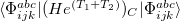 , as a denominator. For the reference (e.g., a ground-state CCSD wave function), the (fT) and (dT) corrections are identical to the CCSD(2)
 and CR-CCSD(T)
 corrections of Piecuch and co-workers [355].
The EOM-SF-CCSD(dT) and EOM-SF-CCSD(fT) methods yield a systematic improvement over EOM-SF-CCSD bringing the errors below 1 kcal/mol. For theoretical background and detailed benchmarks, see Ref. Manohar:2008.
Similar corrections are available for EOM-IP-CCSD [476], where triples correspond to excitations and EOM-EA-CCSD, where triples correspond to  excitations.
6.7.23 Job Control for Non-Iterative Triples Corrections
Triples corrections are requested by using METHOD or EOM_CORR:
METHOD
Specifies the calculation method.
TYPE:
STRING
DEFAULT:
No default value
OPTIONS:
EOM-CCSD(DT)
EOM-CCSD(dT), available for EE, SF, and IP
EOM-CCSD(FT)
EOM-CCSD(fT), available for EE, SF, IP, and EA
EOM-CCSD(ST)
EOM-CCSD(sT), available for IP
RECOMMENDATION:
None
EOM_CORR
Specifies the correlation level.
TYPE:
STRING
DEFAULT:
None
No correction will be computed
OPTIONS:
SD(DT)
EOM-CCSD(dT), available for EE, SF, and IP
SD(FT)
EOM-CCSD(fT), available for EE, SF, IP, and EA
SD(ST)
EOM-CCSD(sT), available for IP
RECOMMENDATION:
None
6.7.24 Examples
Example 6.163 EOM-EE-CCSD(fT) calculation of CH
$molecule
   1 1
   C
   H  C CH

   CH  = 2.137130
$end

$rem
   INPUT_BOHR             true
   METHOD                 eom-ccsd(ft)
   BASIS                  general
   EE_STATES              [1,0,1,1]
   EOM_DAVIDSON_MAX_ITER  60  increase number of Davidson iterations
$end

$basis
 H   0
 S   3  1.00
       19.24060000         0.3282800000E-01
       2.899200000         0.2312080000
      0.6534000000         0.8172380000
 S   1  1.00
      0.1776000000          1.000000000
 S   1  1.00
      0.0250000000          1.000000000
 P   1  1.00
       1.00000000          1.00000000
 ****
 C   0
 S   6  1.00
       4232.610000         0.2029000000E-02
       634.8820000         0.1553500000E-01
       146.0970000         0.7541100000E-01
       42.49740000         0.2571210000
       14.18920000         0.5965550000
       1.966600000         0.2425170000
 S   1  1.00
       5.147700000          1.000000000
 S   1  1.00
      0.4962000000          1.000000000
 S   1  1.00
      0.1533000000          1.000000000
 S   1  1.00
      0.0150000000          1.000000000
 P   4  1.00
       18.15570000         0.1853400000E-01
       3.986400000         0.1154420000
       1.142900000         0.3862060000
      0.3594000000         0.6400890000
 P   1  1.00
      0.1146000000          1.000000000
 P   1  1.00
      0.0110000000          1.000000000
 D   1  1.00
      0.750000000          1.00000000
 ****
$end
Example 6.164 EOM-SF-CCSD(dT) calculations of methylene
$molecule
   0 3
   C
   H 1 CH
   H 1 CH 2 HCH

   CH  = 1.07
   HCH = 111.0
$end

$rem
   METHOD            eom-ccsd(dt)
   BASIS             6-31G
   SF_STATES         [2,0,0,2]
   N_FROZEN_CORE     1
   N_FROZEN_VIRTUAL  1
$end
Example 6.165 EOM-IP-CCSD(dT) calculations of Mg
$molecule
   0 1
   Mg    0.000000     0.000000    0.000000
$end

$rem
   JOBTYPE      sp
   METHOD       eom-ccsd(dt)
   BASIS        6-31g
   IP_STATES    [1,0,0,0,0,1,1,1]
$end
6.7.25 Potential Energy Surface Crossing Minimization
Potential energy surface crossing optimization procedure finds energy minima on crossing seams. On the seam, the potential surfaces are degenerated in the subspace perpendicular to the plane defined by two vectors: the gradient difference
 |
(6.55) |
and the derivative coupling
 |
(6.56) |
At this time Q-Chem is unable to locate crossing minima for states which have non-zero derivative coupling. Fortunately, often this is not the case. Minima on the seams of conical intersections of states of different multiplicity can be found as their derivative coupling is zero. Minima on the seams of intersections of states of different point group symmetry can be located as well.
To run a PES crossing minimization, CCSD and EOM-CCSD methods must be employed for the ground and excited state calculations respectively.
Note: MECP optimization is only available for methods with analytic gradients. Finite-difference evaluation of two gradients is not possible.
6.7.25.1 Job Control Options
XOPT_STATE_1, XOPT_STATE_2
Specify two electronic states the intersection of which will be searched.
TYPE:
[INTEGER, INTEGER, INTEGER]
DEFAULT:
No default value (the option must be specified to run this calculation)
OPTIONS:
[spin, irrep, state]
spin = 0
Addresses states with low spin,
see also EE_SINGLETS or IP_STATES,EA_STATES.
spin = 1
Addresses states with high spin,
see also EE_TRIPLETS.
irrep
Specifies the irreducible representation to which
the state belongs, for
point group symmetry
irrep = 1 for
, irrep = 2 for
irrep = 3 for
state
Specifies the state number within the irreducible
representation, state = 1 means the lowest excited
state, state = 2 is the second excited state, etc..
0, 0, -1
Ground state.
RECOMMENDATION:
Only intersections of states with different spin or symmetry can be calculated at this time.
Note: The spin can only be specified when using closed-shell RHF references. In the case of open-shell references all states are treated together, see also EE_STATES. E.g., in SF calculations use spin=0 regardless of what is the actual multiplicity of the target state.
XOPT_SEAM_ONLY
Orders an intersection seam search only, no minimization is to perform.
TYPE:
LOGICAL
DEFAULT:
FALSE
OPTIONS:
TRUE
Find a point on the intersection seam and stop.
FALSE
Perform a minimization of the intersection seam.
RECOMMENDATION:
In systems with a large number of degrees of freedom it might be useful to locate the seam first setting this option to TRUE and use that geometry as a starting point for the minimization.
6.7.25.2 Examples
Example 6.166 Minimize the intersection of Ã A
A and
and  B states of the NO
 molecule using EOM-IP-CCSD method
$molecule
   -1  1
   N1
   O2  N1  rno
   O3  N1  rno  O2  aono

   rno  = 1.3040
   aono = 106.7
$end

$rem
   JOBTYPE                opt         Optimize the intersection seam
   UNRESTRICTED           true
   METHOD                 eom-ccsd
   BASIS                  6-31g
   IP_STATES              [1,0,1,0]   C2v point group symmetry
   EOM_FAKE_IPEA          1
   XOPT_STATE_1           [0,1,1]     1A1 low spin state
   XOPT_STATE_2           [0,3,1]     1B1 low spin state
   GEOM_OPT_TOL_GRADIENT  30          Tighten gradient tolerance
$END
Example 6.167 Minimize the intersection of Ã B and A states of the N
 ion using EOM-CCSD method
$molecule
   1 1
   N1
   N2 N1 rnn
   N3 N2 rnn N1 annn

   rnn=1.46
   annn=70.0
$end

$rem
   JOBTYPE                opt
   METHOD                 eom-ccsd
   BASIS                  6-31g
   EE_SINGLES             [0,2,0,2]   C2v point group symmetry
   XOPT_STATE_1           [0,4,1]     1B2 low spin state
   XOPT_STATE_2           [0,2,2]     2A2 low spin state
   XOPT_SEAM_ONLY         true        Find the seam only
   GEOM_OPT_TOL_GRADIENT  100
$end

$opt
CONSTRAINT                Set constraints on the N-N bond lengths
   stre  1  2  1.46
   stre  2  3  1.46
ENDCONSTRAINT
$end

@@@

$molecule
   READ
$end

$rem
   JOBTYPE                opt         Optimize the intersection seam
   METHOD                 eom-ccsd
   BASIS                  6-31g
   EE_SINGLETS            [0,2,0,2]
   XOPT_STATE_1           [0,4,1]
   XOPT_STATE_2           [0,2,2]
   GEOM_OPT_TOL_GRADIENT  30
$end
6.7.26 Dyson Orbitals for Ionization States within the EOM-CCSD Formalism
Dyson orbitals can be used to compute total photodetachment/photoionization cross-sections, as well as angular distribution of photoelectrons. A Dyson orbital is the overlap between the N-electron molecular wave function and the N-1/N+1 electron wave function of the corresponding cation/anion:
 |
|
 |
(6.57) | ||
 |
|
 |
(6.58) |
For the Hartree-Fock wave functions and within Koopmans’ approximation, these are just the canonical HF orbitals. For correlated wave functions, Dyson orbitals are linear combinations of the reference molecular orbitals:
 |
|
 |
(6.59) | ||
 |
|
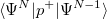 |
(6.60) | ||
|
|
 |
(6.61) |
The calculation of Dyson orbitals is straightforward within the EOM-IP/EA-CCSD methods, where cation/anion and initial molecule states are defined with respect to the same MO basis. Since the left and right CC vectors are not the same, one can define correspondingly two Dyson orbitals (left and right):
 |
|
 |
(6.62) | ||
 |
|
 |
(6.63) |
The norm of these orbitals is proportional to the one-electron character of the transition.
Dyson orbitals also offer qualitative insight visualizing the difference between molecular and ionized/attached states. In ionization/photodetachment processes, these orbitals can be also interpreted as the wave function of the leaving electron. For additional details, see Refs. Oana:2007,Oana:2009.
6.7.26.1 Dyson Orbitals Job Control
The calculation of Dyson orbitals is implemented for the ground (reference) and excited states ionization/electron attachment. To obtain the ground state Dyson orbitals one needs to run an EOM-IP/EA-CCSD calculation, request transition properties calculation by setting CC_TRANS_PROP=TRUE and CC_DO_DYSON = TRUE. The Dyson orbitals decomposition in the MO basis is printed in the output, for all transitions between the reference and all IP/EA states. At the end of the file, also the coefficients of the Dyson orbitals in the AO basis are available.
Two implementations of Dyson orbitals are currently available: (i) the original implementation in CCMAN; and (ii) new implementation in CCMAN2. The CCMAN implementation is using a diffuse orbital trick (i.e., EOM_FAKE_IPEA will be automatically set to TRUE in these calculations). Note: this implementation has a bug affecting the values of norms of Dyson orbitals (the shapes are correct); thus, using this code is strongly discouraged. The CCMAN2 implementation has all types of initial states available: Dyson orbitals from ground CC, excited EOM-EE, and spin-flip EOM-SF states; it is fully compatible with all helper features for EOM calculations, like FNO, RI, Cholesky decomposition. The CCMAN2 implementation can utilize user-specified EOM guess (using EOM_USER_GUESS keyword and $eom_user_guess section), which is recommended for highly excited states (such as core-ionized states). In addition, CCMAN2 can calculate Dyson orbitals involving meta-stable states (see Section 6.7.5).
For calculating Dyson orbitals between excited or spin-flip states from the reference configuration and IP/EA states, same CC_TRANS_PROP = TRUE and CC_DO_DYSON = TRUE keywords have to be added to the combination of usual EOM-IP/EA-CCSD and EOM-EE-CCSD or EOM-SF-CCSD calculations (however, note separate keyword CC_DO_DYSON_EE = TRUE for CCMAN). The IP_STATES keyword is used to specify the target ionized states. The attached states are specified by EA_STATES. The EA-SF states are specified by EOM_EA_BETA. The excited (or spin-flipped) states are specified by EE_STATES and SF_STATES. The Dyson orbital decomposition in MO and AO bases is printed for each EE/SF-IP/EA pair of states first for reference, then for all excited states in the order: CC - IP/EA1, CC - IP/EA2, , EE/SF1 - IP/EA1, EE/SF1 - IP/EA2,, EE/SF2 - IP/EA1, EE/SF2 - IP/EA2,, and so on. CCMAN implementation keeps reference transitions separate, in accordance with separating keywords.
CC_DO_DYSON
CCMAN2: starts all types of Dyson orbitals calculations. Desired type is determined by requesting corresponding EOM-XX transitions CCMAN: whether the reference-state Dyson orbitals will be calculated for EOM-IP/EA-CCSD calculations.
TYPE:
LOGICAL
DEFAULT:
FALSE (the option must be specified to run this calculation)
OPTIONS:
TRUE/FALSE
RECOMMENDATION:
none
CC_DO_DYSON_EE
Whether excited-state or spin-flip state Dyson orbitals will be calculated for EOM-IP/EA-CCSD calculations with CCMAN.
TYPE:
LOGICAL
DEFAULT:
FALSE (the option must be specified to run this calculation)
OPTIONS:
TRUE/FALSE
RECOMMENDATION:
none
Dyson orbitals can be also plotted using IANLTY = 200 and the $plots utility. Only the sizes of the box need to be specified, followed by a line of zeros:
$plots
comment
   10   -2   2
   10   -2   2
   10   -2   2
   0     0   0    0
$plots
All Dyson orbitals on the Cartesian grid will be written in the resulting plot.mo file (only CCMAN). For RHF(UHF) reference, the columns order in plot.mo is: 
In addition, setting the MAKE_CUBE_FILES keyword to TRUE will create cube files for Dyson orbitals which can be viewed with VMD or other programs (see Section 10.5.4 for details). This option is available for CCMAN and CCMAN2. The Dyson orbitals will be written to files mo.1.cube, mo.2.cube, in the order  . For meta-stable states, the real and imaginary parts of the Dyson orbitals are written to separate files in the order
Other means of visualization (e.g., with MOLDEN_FORMAT = TRUE or GUI = 2) are currently not available.
6.7.26.2 Examples
Example 6.168 Plotting grd-ex and ex-grd state Dyson orbitals for ionization of the oxygen molecule. The target states of the cation are A and B
and B . Works for CCMAN only.
$molecule
   0 3
   O    0.000  0.000  0.000
   O    1.222  0.000  0.000
$end

$rem
   BASIS          6-31G*
   METHOD         eom-ccsd
   IP_STATES      [1,0,0,0,0,0,1,0] Target EOM-IP states
   CC_TRANS_PROP  true  request transition OPDMs to be calculated
   CC_DO_DYSON    true  calculate Dyson orbitals
   IANLTY         200
$end

$plots
plots excited states densities and trans densities
   10   -2   2
   10   -2   2
   10   -2   2
   0     0   0    0
$plots
Example 6.169 Plotting ex-ex state Dyson orbitals between the 1st  excited state of the HO radical and the the 1st A and A excited states of HO. Works for CCMAN only.
$molecule
   -1 1
   H    0.000   0.000  0.000
   O    1.000   0.000  0.000
$end

$rem
   METHOD             eom-ccsd
   BASIS              6-31G*
   IP_STATES          [1,0,0,0]  states of HO radical
   EE_STATES          [1,1,0,0]  excited states of HO-
   CC_TRANS_PROP      true       calculate transition properties
   CC_DO_DYSON_EE     true       calculate Dyson orbitals for ionization from ex. states
   IANLTY             200
$end

$plots
plot excited states densities and trans densities
   10   -2   2
   10   -2   2
   10   -2   2
   0     0   0    0
$plots
Example 6.170 Dyson orbitals for ionization of CO molecule; A and B ionized states requested.
$molecule
   0 1
   O
   C  O  1.131
$end

$rem
   CORRELATION           CCSD
   BASIS                 cc-pVDZ
   PURECART              111        5d, will be required for ezDyson
   IP_STATES             [1,0,1,0]  (A1,A2,B1,B2)
   CCMAN2                true
   CC_DO_DYSON           true
   CC_TRANS_PROP         true       necessary for Dyson orbitals job
   PRINT_GENERAL_BASIS   true       will be required for ezDyson
$end
Example 6.171 Dyson orbitals for ionization of HO; core (A) state requested — ionization from O(1s).
$molecule
   0 1
   O
   H1  O  0.955
   H2  O  0.955  H1  104.5
$end

$rem
   CORRELATION           CCSD
   BASIS                 cc-pVTZ
   PURECART              111        5d, will be required for ezDyson
   IP_STATES             [1,0,0,0]  (A1,A2,B1,B2)
   EOM_USER_GUESS        1          on, further defined in $eom_user_guess
   CCMAN2                true
   CC_DO_DYSON           true
   CC_TRANS_PROP         true       necessary for Dyson orbitals job
   PRINT_GENERAL_BASIS   true       will be required for ezDyson
$end

$eom_user_guess
   1
$end
Example 6.172 Dyson orbitals for ionization of NO molecule using EOM-EA and a closed-shell cation reference; A and B states requested.
$molecule
   +1 1
   N   0.00000  0.00000  0.00000
   O   0.00000  0.00000  1.02286
$end

$rem
   CORRELATION            CCSD
   BASIS                  aug-cc-pVTZ
   PURECART               111       5d, will be required for ezDyson
   EA_STATES              [1,0,0,1] (A1,A2,B1,B2)
   CCMAN2                 true
   CC_DO_DYSON            true
   CC_TRANS_PROP          true      necessary for Dyson orbitals job
   PRINT_GENERAL_BASIS    true      will be required for ezDyson
$end
Example 6.173 Dyson orbitals for ionization of triplet O and O at slightly stretched (relative to the equilibrium O geometry); B states are requested.
$comment
   EOM-IP-CCSD/6-311+G* and EOM-EA-CCSD/6-311+G* levels of theory,
   UHF reference.  Start from O2:
    1) detach electron - ionization of neutral (alpha IP).
    2) attach electron, use EOM-EA w.f. as initial state
       - ionization of anion (beta EA).
$end

$molecule
   0 3
   O   0.00000  0.00000  0.00000
   O   0.00000  0.00000  1.30000
$end

$rem
   CORRELATION           CCSD
   BASIS                 6-311(3+)G*
   PURECART              2222          6d, will be required for ezDyson
   EOM_IP_ALPHA          [0,0,0,1,0,0,0,0]  (Ag,B1g,B2g,B3g,Au,B1u,B2u,B3u)
   EOM_EA_BETA           [0,0,0,1,0,0,0,0]  (Ag,B1g,B2g,B3g,Au,B1u,B2u,B3u)
   CCMAN2                true
   CC_DO_DYSON           true
   CC_TRANS_PROP         true          necessary for Dyson orbitals job
   PRINT_GENERAL_BASIS   true          will be required for ezDyson
$end
Example 6.174 Dyson orbitals for detachment from the meta-stable  state of N.
$molecule
   0 1
   N   0.0   0.0    0.55
   N   0.0   0.0   -0.55
   GH  0.0   0.0    0.0
$end

$rem
   METHOD            EOM-CCSD
   EA_STATES         [0,0,2,0,0,0,0,0]
   CC_MEMORY         5000
   MEM_STATIC        1000
   BASIS             GEN
   COMPLEX_CCMAN     TRUE
   CC_TRANS_PROP     TRUE
   CC_DO_DYSON       TRUE
   MAKE_CUBE_FILES   TRUE
   IANLTY            200
$end

$complex_ccman
   CS_HF 1
   CAP_TYPE 1
   CAP_X 2760
   CAP_Y 2760
   CAP_Z 4880
   CAP_ETA 400
$end

$plots
plot Dyson orbitals
   50 -10.0 10.0
   50 -10.0 10.0
   50 -10.0 10.0
   0 0 0 0
$end

$basis
N    0
S    8    1.000000
   1.14200000E+04    5.23000000E-04
   1.71200000E+03    4.04500000E-03
   3.89300000E+02    2.07750000E-02
   1.10000000E+02    8.07270000E-02
   3.55700000E+01    2.33074000E-01
   1.25400000E+01    4.33501000E-01
   4.64400000E+00    3.47472000E-01
   5.11800000E-01   -8.50800000E-03
S    8    1.000000
   1.14200000E+04   -1.15000000E-04
   1.71200000E+03   -8.95000000E-04
   3.89300000E+02   -4.62400000E-03
   1.10000000E+02   -1.85280000E-02
   3.55700000E+01   -5.73390000E-02
   1.25400000E+01   -1.32076000E-01
   4.64400000E+00   -1.72510000E-01
   5.11800000E-01    5.99944000E-01
S    1    1.000000
   1.29300000E+00    1.00000000E+00
S    1    1.000000
   1.78700000E-01    1.00000000E+00
P    3    1.000000
   2.66300000E+01    1.46700000E-02
   5.94800000E+00    9.17640000E-02
   1.74200000E+00    2.98683000E-01
P    1    1.000000
   5.55000000E-01    1.00000000E+00
P    1    1.000000
   1.72500000E-01    1.00000000E+00
D    1    1.000000
   1.65400000E+00    1.00000000E+00
D    1    1.000000
   4.69000000E-01    1.00000000E+00
F    1    1.000000
   1.09300000E+00    1.00000000E+00
S    1    1.000000
   5.76000000E-02    1.00000000E+00
P    1    1.000000
   4.91000000E-02    1.00000000E+00
D    1    1.000000
   1.51000000E-01    1.00000000E+00
F    1    1.000000
   3.64000000E-01    1.00000000E+00
****
GH   0
S    1    1.000000
   2.88000000E-02    1.00000000E+00
S    1    1.000000
   1.44000000E-02    1.00000000E+00
S    1    1.000000
   0.72000000E-02    1.00000000E+00
S    1    1.000000
   0.36000000E-02    1.00000000E+00
S    1    1.000000
   0.18000000E-02    1.00000000E+00
S    1    1.000000
   0.09000000E-02    1.00000000E+00
P    1    1.000000
   2.45000000E-02    1.00000000E+00
P    1    1.000000
   1.22000000E-02    1.00000000E+00
P    1    1.000000
   0.61000000E-02    1.00000000E+00
P    1    1.000000
   0.305000000E-02    1.00000000E+00
P    1    1.000000
   0.152500000E-02    1.00000000E+00
P    1    1.000000
   0.076250000E-02    1.00000000E+00
D    1    1.000000
   0.755000000E-01    1.00000000E+00
D    1    1.000000
   0.377500000E-01    1.00000000E+00
D    1    1.000000
   0.188750000E-01    1.00000000E+00
D    1    1.000000
   0.094375000E-01    1.00000000E+00
D    1    1.000000
   0.047187500E-01    1.00000000E+00
D    1    1.000000
   0.023593750E-01    1.00000000E+00
****
$end
Example 6.175 Dyson orbitals for ionization of formaldehyde from the first excited state AND from the ground state
$molecule
   0 1
   O     1.535338855      0.000000000     -0.438858006
   C     1.535331598     -0.000007025      0.767790994
   H     1.535342484      0.937663512      1.362651452
   H     1.535342484     -0.937656488      1.362672535
$end

$rem
   CORRELATION           CCSD
   BASIS                 6-31G*
   PURECART              2222    6d, will be required for ezDyson
   CCMAN2                true    new Dyson code
   EE_STATES             [1]
   EOM_IP_ALPHA          [1]
   EOM_IP_BETA           [1]
   CC_TRANS_PROP         true    necessary for Dyson orbitals job
   CC_DO_DYSON           true
   PRINT_GENERAL_BASIS   true    will be required for ezDyson
$end
Example 6.176 Dyson orbitals for core ionization of Li atom use Li as a reference, get neutral atom via EOM-EA get 1st excitation for the cation via EOM-EE totally: core ionization AND 1st ionization of Li atom
$molecule
   +1 1
   Li   0.00000  0.00000  0.00000
$end

$rem
   CORRELATION            CCSD
   BASIS                  6-311+G*
   PURECART               2222          6d, will be required for ezDyson
   CCMAN2                 true          new Dyson code
   EE_STATES              [1,0,0,0,0,0,0,0]
   EA_STATES              [1,0,0,0,0,0,0,0]
   EOM_NGUESS_SINGLES     5             to converge to the lowest EA state
   CC_TRANS_PROP          true          necessary for Dyson orbitals job
   CC_DO_DYSON            true
   PRINT_GENERAL_BASIS    true          will be required for ezDyson
$end
Example 6.177 Dyson orbitals for ionization of CH2 from high-spin triplet reference and from the lowest SF state
$molecule
   0 3
   C
   H  1 rCH
   H  1 rCH 2 aHCH

   rCH    = 1.1167
   aHCH   = 102.07
$end

$rem
   CORRELATION           CCSD
   BASIS                 6-31G*
   PURECART              2222    6d, will be required for ezDyson
   SCF_GUESS             core
   CCMAN2                true    new Dyson code
   CC_SYMMETRY           false
   SF_STATES             [1]
   EOM_IP_ALPHA          [2]     one should be careful to request
   EOM_EA_BETA           [2]     meaningful spin for EA/IP state(s)
   CC_TRANS_PROP         true    necessary for Dyson orbitals job
   CC_DO_DYSON           true
   PRINT_GENERAL_BASIS   true    will be required for ezDyson
$end
6.7.27 Interpretation of EOM/CI Wave Functions and Orbital Numbering
Analysis of the leading wave function amplitudes is always necessary for determining the character of the state (e.g., HOMO-LUMO excitation, open-shell diradical, etc.). The CCMAN module print out leading EOM/CI amplitudes using its internal orbital numbering scheme, which is printed in the beginning. The typical CCMAN EOM-CCSD output looks like:
Root 1 Conv-d yes Tot Ene= -113.722767530 hartree (Ex Ene 7.9548 eV),
U1^2=0.858795, U2^2=0.141205 ||Res||=4.4E-07
Right U1:
       Value                   i            ->    a
       0.5358                  7( B2  ) B   ->   17( B2  ) B
       0.5358                  7( B2  ) A   ->   17( B2  ) A
      -0.2278                  7( B2  ) B   ->   18( B2  ) B
      -0.2278                  7( B2  ) A   ->   18( B2  ) A
This means that this state is derived by excitation from occupied orbital #7 (which has symmetry) to virtual orbital #17 (which is also of symmetry). The two leading amplitudes correspond to  and
and  excitation (the spin part is denoted by or
  ). The orbital numbering for this job is defined by the following map:
The orbitals are ordered and numbered as follows:
Alpha orbitals:
Number  Energy    Type    Symmetry  ANLMAN number  Total number:
  0    -20.613     AOCC      A1      1A1     1
  1    -11.367     AOCC      A1      2A1     2
  2     -1.324     AOCC      A1      3A1     3
  3     -0.944     AOCC      A1      4A1     4
  4     -0.600     AOCC      A1      5A1     5
  5     -0.720     AOCC      B1      1B1     6
  6     -0.473     AOCC      B1      2B1     7
  7     -0.473     AOCC      B2      1B2     8

  0      0.071     AVIRT     A1      6A1     9
  1      0.100     AVIRT     A1      7A1     10
  2      0.290     AVIRT     A1      8A1     11
  3      0.327     AVIRT     A1      9A1     12
  4      0.367     AVIRT     A1     10A1     13
  5      0.454     AVIRT     A1     11A1     14
  6      0.808     AVIRT     A1     12A1     15
  7      1.196     AVIRT     A1     13A1     16
  8      1.295     AVIRT     A1     14A1     17
  9      1.562     AVIRT     A1     15A1     18
 10      2.003     AVIRT     A1     16A1     19
 11      0.100     AVIRT     B1      3B1     20
 12      0.319     AVIRT     B1      4B1     21
 13      0.395     AVIRT     B1      5B1     22
 14      0.881     AVIRT     B1      6B1     23
 15      1.291     AVIRT     B1      7B1     24
 16      1.550     AVIRT     B1      8B1     25
 17      0.040     AVIRT     B2      2B2     26
 18      0.137     AVIRT     B2      3B2     27
 19      0.330     AVIRT     B2      4B2     28
 20      0.853     AVIRT     B2      5B2     29
 21      1.491     AVIRT     B2      6B2     30
The first column is CCMAN’s internal numbering (e.g., 7 and 17 from the example above). This is followed by the orbital energy, orbital type (frozen, restricted, active, occupied, virtual), and orbital symmetry. Note that the orbitals are blocked by symmetries and then ordered by energy within each symmetry block, (i.e., first all occupied , then all  , etc.), and numbered starting from 0. The occupied and virtual orbitals are numbered separately, and frozen orbitals are excluded from CCMAN numbering. The two last columns give numbering in terms of the final ANLMAN printout (starting from 1), e.g., our occupied orbital #7 will be numbered as 1 in the final printout. The last column gives the absolute orbital number (all occupied and all virtuals together, starting from 1), which is often used by external visualization routines.
CCMAN2 numbers orbitals by their energy within each irrep keeping the same numbering for occupied and virtual orbitals. This numbering is exactly the same as in the final printout of the SCF wave function analysis. Orbital energies are printed next to the respective amplitudes. For example, a typical CCMAN2 EOM-CCSD output will look like that:
 EOMEE-CCSD transition 2/A1
 Total energy = -75.87450159 a.u.  Excitation energy = 11.2971 eV.
 R1^2 = 0.9396  R2^2 = 0.0604  Res^2 = 9.51e-08

 Amplitude    Orbitals with energies
  0.6486       1 (B2) A                  ->    2 (B2) A
              -0.5101                          0.1729
  0.6486       1 (B2) B                  ->    2 (B2) B
              -0.5101                          0.1729
 -0.1268       3 (A1) A                  ->    4 (A1) A
              -0.5863                          0.0404
 -0.1268       3 (A1) B                  ->    4 (A1) B
              -0.5863                          0.0404
which means that for this state, the leading EOM amplitude corresponds to the transition from the first b orbital (orbital energy  ) to the second b orbital (orbital energy 0.1729).