6.2 Uncorrelated Wave Function Methods

Q-Chem includes several excited state methods which do not incorporate correlation: CIS, XCIS and RPA. These methods are sufficiently inexpensive that calculations on large molecules are possible, and are roughly comparable to the HF treatment of the ground state in terms of performance. They tend to yield qualitative rather than quantitative insight. Excitation energies tend to exhibit errors on the order of an electron volt, consistent with the neglect of electron correlation effects, which are generally different in the ground state and the excited state.

6.2.1 Single Excitation Configuration Interaction (CIS)

The derivation of the CI-singles [394, 395] energy and wave function begins by selecting the HF single-determinant wave function as reference for the ground state of the system:

$\begin{equation} \label{eq600} \Psi _{\ensuremath{\mathrm{HF}}} =\frac{1}{\sqrt {n!} }\det \left\{ {\chi _1 \chi { }_2\cdots \chi _ i \chi { }_ j\cdots \chi _ n } \right\} \end{equation}$

(6.1)

where $n$ is the number of electrons, and the spin orbitals

$\begin{equation} \label{eq601} \chi _ i =\sum \limits _\mu ^ N {c_{\mu i} \phi _\mu } \end{equation}$

(6.2)

are expanded in a finite basis of $N$ atomic orbital basis functions. Molecular orbital coefficients $\{ c_{\mu i}\}$ are usually found by SCF procedures which solve the Hartree-Fock equations

$\begin{equation} \label{eq602} \ensuremath{\mathbf{FC}} = \bm@general \boldmath \m@ne \mv@bold \bm@command {\varepsilon }\ensuremath{\mathbf{SC}} \; , \end{equation}$

(6.3)

where S is the overlap matrix, C is the matrix of molecular orbital coefficients, ${\varepsilon }$ is a diagonal matrix of orbital eigenvalues and F is the Fock matrix with elements

$\begin{equation} \label{eq603} F_{\mu \upsilon } =H_{\mu \upsilon } +\sum \limits _{\lambda \sigma } {\sum \limits _ i {c_{\mu i} c_{\upsilon i} \left( {\mu \lambda } \right.\vert \vert \left. {\upsilon \sigma } \right)} } \end{equation}$

(6.4)

involving the core Hamiltonian and the anti-symmetrized two-electron integrals

$\begin{equation} (\mu \mu ||\lambda \sigma ) = \int \int \phi _\mu (\mathbf{r}_1^{}) \phi _\nu (\mathbf{r}_2^{}) \left(\frac{1}{r_{12}^{}}\right) \bigl [ \phi _\lambda (\mathbf{r}_1^{}) \phi _\sigma (\mathbf{r}_2^{}) - \phi _\sigma (\mathbf{r}_1^{}) \phi _\lambda (\mathbf{r}_2^{}) \bigr ] \; d\mathbf{r}_1^{} \, d\mathbf{r}_2^{} \end{equation}$

(6.5)

On solving Eq. (6.3), the total energy of the ground state single determinant can be expressed as

$\begin{equation} \label{eq605} E_{\ensuremath{\mathrm{HF}}} =\sum \limits _{\mu \upsilon } {P_{\mu \upsilon }^{\ensuremath{\mathrm{HF}}} H_{\mu \upsilon } } +\frac{1}{2}\sum \limits _{\mu \upsilon \lambda \sigma } {P_{\mu \upsilon }^{\ensuremath{\mathrm{HF}}} P_{\lambda \sigma }^{\ensuremath{\mathrm{HF}}} \left( {\mu \lambda } \right.\vert \vert \left. {\upsilon \sigma } \right)} +V_{\ensuremath{\mathrm{nuc}}} \end{equation}$

(6.6)

where $P^{\ensuremath{\mathrm{HF}}}$ is the HF density matrix and $V_{\ensuremath{\mathrm{nuc}}}$ is the nuclear repulsion energy.

Equation (6.1) represents only one of many possible determinants made from orbitals of the system; there are in fact $n(N-n)$ possible singly substituted determinants constructed by replacing an orbital occupied in the ground state ( $i$ , $j$ , $k,\ldots$ ) with an orbital unoccupied in the ground state ( $a$ , $b$ , $c, \ldots$ ). Such wave functions and energies can be written

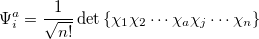$\begin{equation} \label{eq606} \Psi _ i^ a =\frac{1}{\sqrt {n!} }\det \left\{ {\chi _1 \chi { }_2\cdots \chi _ a \chi { }_ j\cdots \chi _ n } \right\} \end{equation}$

(6.7)

$\begin{equation} \label{eq607} E_{ia} =E_{\ensuremath{\mathrm{HF}}} +\varepsilon _ a -\varepsilon _ i -\left( {ia} \right.\vert \vert \left. {ia} \right) \end{equation}$

(6.8)

where we have introduced the anti-symmetrized two-electron integrals in the molecular orbital basis

$\begin{equation} \label{eq608} \left( {pq} \right.\vert \vert \left. {rs} \right)=\sum \limits _{\mu \upsilon \lambda \sigma } {c_{\mu p} c_{\upsilon q} c_{\lambda r} c_{\sigma s} \left( {\mu \lambda } \right.\vert \vert \left. {\upsilon \sigma } \right)} \end{equation}$

(6.9)

These singly excited wave functions and energies could be considered crude approximations to the excited states of the system. However, determinants of the form Eq. (6.7) are deficient in that they:

do not yield pure spin states
resemble more closely ionization rather than excitation
are not appropriate for excitation into degenerate states

These deficiencies can be partially overcome by representing the excited state wave function as a linear combination of all possible singly excited determinants,

$\begin{equation} \label{eq609} \Psi _{\ensuremath{\mathrm{CIS}}} =\sum \limits _{ia} {a_ i^ a \Psi _ i^ a } \end{equation}$

(6.10)

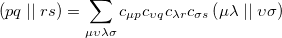
where the coefficients $\{ a_{ia}\}$ can be obtained by diagonalizing the many-electron Hamiltonian, A, in the space of all single substitutions. The appropriate matrix elements are:

$\begin{equation} \label{eq:orbital-Hessian} A_{ia,jb} =\left\langle {\Psi _ i^ a } \right|H\left| {\Psi _ j^ b } \right\rangle =(\varepsilon _ a -\varepsilon _ j )\delta _{ij} \delta _{ab} -\left( {ja} \right.\vert \vert \left. {ib} \right) \end{equation}$

(6.11)

According to Brillouin’s, theorem single substitutions do not interact directly with a reference HF determinant, so the resulting eigenvectors from the CIS excited state represent a treatment roughly comparable to that of the HF ground state. The excitation energy is simply the difference between HF ground state energy and CIS excited state energies, and the eigenvectors of A correspond to the amplitudes of the single-electron promotions.

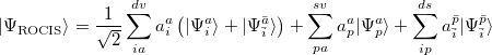
CIS calculations can be performed in Q-Chem using restricted (RCIS) [394, 395], unrestricted (UCIS), or restricted open shell (ROCIS) [396] spin orbitals.

6.2.2 Random Phase Approximation (RPA)

The Random Phase Approximation (RPA) [397, 398], also known as time-dependent Hartree-Fock (TD-HF) theory, is an alternative to CIS for uncorrelated calculations of excited states. It offers some advantages for computing oscillator strengths, e.g., exact satisfaction of the Thomas-Reike-Kuhn sum rule [399], and is roughly comparable in accuracy to CIS for singlet excitation energies, but is inferior for triplet states. RPA energies are non-variational, and in moving around on excited-state potential energy surfaces, this method can occasionally encounter singularities that prevent numerical solution of the underlying equations [400], whereas such singularities are mathematically impossible in CIS calculations.

6.2.3 Extended CIS (XCIS)

The motivation for the extended CIS procedure (XCIS) [401] stems from the fact that ROCIS and UCIS are less effective for radicals that CIS is for closed shell molecules. Using the attachment/detachment density analysis procedure [402], the failing of ROCIS and UCIS methodologies for the nitromethyl radical was traced to the neglect of a particular class of double substitution which involves the simultaneous promotion of an $\alpha$ spin electron from the singly occupied orbital and the promotion of a $\beta$ spin electron into the singly occupied orbital. The spin-adapted configurations

$\begin{equation} \label{eq611} \left| {\tilde{\Psi }_ i^ a (1)} \right\rangle =\frac{1}{\sqrt 6 }\left( |\Psi _{\bar{i}}^{\bar{a}}\rangle -|\Psi _ i^ a\rangle \right)+\frac{2}{\sqrt 6 }|\Psi _{p\bar{i}}^{a\bar{p}}\rangle \end{equation}$

(6.12)

are of crucial importance. (Here, $a, b, c, \ldots$ are virtual orbitals; $i, j, k, \ldots$ are occupied orbitals; and $p, q, r, \ldots$ are singly-occupied orbitals.) It is quite likely that similar excitations are also very significant in other radicals of interest.

The XCIS proposal, a more satisfactory generalization of CIS to open shell molecules, is to simultaneously include a restricted class of double substitutions similar to those in Eq. (6.12). To illustrate this, consider the resulting orbital spaces of an ROHF calculation: doubly occupied ( $d$ ), singly occupied ( $s$ ) and virtual ( $v$ ). From this starting point we can distinguish three types of single excitations of the same multiplicity as the ground state: $d \rightarrow s$ , $s \rightarrow v$ and $d \rightarrow v$ . Thus, the spin-adapted ROCIS wave function is

$\begin{equation} \label{eq612} \left| {\Psi _{\ensuremath{\mathrm{ROCIS}}} } \right\rangle =\frac{1}{\sqrt 2 }\sum _{ia}^{dv} a_ i^ a \left( |\Psi _ i^ a\rangle +|\Psi _{\bar{i}}^{\bar{a}} \rangle \right) +\sum _{pa}^{sv} a_ p^ a |\Psi _ p^ a\rangle +\sum _{ip}^{ds} a_{\bar{i}}^{\bar{p}} |\Psi _{\bar{i}}^{\bar{p}}\rangle \end{equation}$

(6.13)

The extension of CIS theory to incorporate higher excitations maintains the ROHF as the ground state reference and adds terms to the ROCIS wave function similar to that of Eq. (6.13), as well as those where the double excitation occurs through different orbitals in the $\alpha$ and $\beta$ space:

$\begin{equation} \label{eq613} \begin{array}{r} \left| {\Psi _{\ensuremath{\mathrm{XCIS}}} } \right\rangle =\frac{1}{\sqrt 2 }{\displaystyle \sum _{ia}^{dv}} a_ i^ a \left( |\Psi _ i^ a\rangle +|\Psi _{\bar{i}}^{\bar{a}}\rangle \right) +{\displaystyle \sum _{pa}^{sv}} a_ p^ a |\Psi _ p^ a\rangle +{\displaystyle \sum _{ip}^{ds}} a_{\bar{i}}^{\bar{p}} |\Psi _{\bar{i}}^{\bar{p}}\rangle \\ +{\displaystyle \sum _{iap}^{dvs}} \tilde{a}_ i^ a (p)|\tilde{\Psi }_ i^ a (p)\rangle +{\displaystyle \sum _{ia,p\ne q}^{dv,ss}} a_{p\bar{i}}^{a\bar{q}} |\Psi _{p\bar{i}}^{a\bar{q}}\rangle \\ \end{array} \end{equation}$

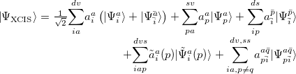(6.14)

XCIS is defined only from a restricted open shell Hartree-Fock ground state reference, as it would be difficult to uniquely define singly occupied orbitals in a UHF wave function. In addition, $\beta$ unoccupied orbitals, through which the spin-flip double excitation proceeds, may not match the half-occupied $\alpha$ orbitals in either character or even symmetry.

For molecules with closed shell ground states, both the HF ground and CIS excited states emerge from diagonalization of the Hamiltonian in the space of the HF reference and singly excited substituted configuration state functions. The XCIS case is different because the restricted class of double excitations included could mix with the ground state and lower its energy. This mixing is avoided to maintain the size consistency of the ground state energy.

With the inclusion of the restricted set of doubles excitations in the excited states, but not in the ground state, it could be expected that some fraction of the correlation energy be recovered, resulting in anomalously low excited state energies. However, the fraction of the total number of doubles excitations included in the XCIS wave function is very small and those introduced cannot account for the pair correlation of any pair of electrons. Thus, the XCIS procedure can be considered one that neglects electron correlation.

The computational cost of XCIS is approximately four times greater than CIS and ROCIS, and its accuracy for open shell molecules is generally comparable to that of the CIS method for closed shell molecules. In general, it achieves qualitative agreement with experiment. XCIS is available for doublet and quartet excited states beginning from a doublet ROHF treatment of the ground state, for excitation energies only.

6.2.4 Spin-Flip Extended CIS (SF-XCIS)

Spin-flip extended CIS (SF-XCIS) [403] is a spin-complete extension of the spin-flip single excitation configuration interaction (SF-CIS) method [404]. The method includes all configurations in which no more than one virtual level of the high spin triplet reference becomes occupied and no more than one doubly occupied level becomes vacant.

SF-XCIS is defined only from a restricted open shell Hartree-Fock triplet ground state reference. The final SF-XCIS wave functions correspond to spin-pure $M_ S=0$ (singlet or triplet) states. The fully balanced treatment of the half-occupied reference orbitals makes it very suitable for applications with two strongly correlated electrons, such as single bond dissociation, systems with important diradical character or the study of excited states with significant double excitation character.

The computational cost of SF-XCIS scales in the same way with molecule size as CIS itself, with a pre-factor 13 times larger.

6.2.5 CIS Analytical Derivatives

While CIS excitation energies are relatively inaccurate, with errors of the order of 1 eV, CIS excited state properties, such as structures and frequencies, are much more useful. This is very similar to the manner in which ground state Hartree-Fock (HF) structures and frequencies are much more accurate than HF relative energies. Generally speaking, for low-lying excited states, it is expected that CIS vibrational frequencies will be systematically 10% higher or so relative to experiment [405, 406, 407]. If the excited states are of pure valence character, then basis set requirements are generally similar to the ground state. Excited states with partial Rydberg character require the addition of one or preferably two sets of diffuse functions.

Q-Chem includes efficient analytical first and second derivatives of the CIS energy [408, 409], to yield analytical gradients, excited state vibrational frequencies, force constants, polarizabilities, and infrared intensities. Analytical gradients can be evaluated for any job where the CIS excitation energy calculation itself is feasible, so that efficient excited-state geometry optimizations and vibrational frequency calculations are possible at the CIS level. In such cases, it is necessary to specify on which Born-Oppenheimer potential energy surface the optimization should proceed, and care must be taken to ensure that the optimization remains on the excited state of interest, as state crossings may occur. (A “state-tracking” algorithm, as discussed in Section 9.6.5, can aid with this.)

Sometimes it is precisely the crossings between Born-Oppenheimer potential energy surfaces (i.e., conical intersections) that are of interest, as these intersections provide pathways for non-adiabatic transitions between electronic states [410, 411]. A feature of Q-Chem that is not otherwise widely available in an analytic implementation [412, 413, 414, 415] (for both CIS and TDDFT) of the non-adiabatic couplings that define the topology around conical intersections. Due to the analytic implementation, these couplings can be evaluated at a cost that is not significantly greater than the cost of a CIS or TDDFT analytic gradient calculation, and the availability of these couplings allows for much more efficient optimization of minimum-energy crossing points along seams of conical intersection, as compared to when only analytic gradients are available [413]. These features, including a brief overview of the theory of conical intersections, can be found in Section 9.6.1.

For CIS vibrational frequencies, a semi-direct algorithm similar to that used for ground-state Hartree-Fock frequencies is available, whose computer time scales as approximately ${\cal {O}}({N^3})$ for large molecules [401]. The main complication associated with analytical CIS frequency calculations is ensuring that Q-Chem has sufficient memory to perform the calculations. Default settings are adequate for many purposes but if a large calculation fails due to a memory limitation, then the following additional information may be useful.

The memory requirements for CIS (and HF) analytic frequencies primarily come from dynamic memory, defined as

dynamic memory = MEM_TOTAL $-$ MEM_STATIC .

This quantity must be large enough to contain several arrays whose size is $3 N_{\rm atoms} N_{\rm basis}^2$ . Meanwhile the value of the $rem variable MEM_STATIC, which obviously reduces the available dynamic memory, must be sufficiently large to permit integral evaluation, else the job may fail. For most purposes, setting MEM_STATIC to about 80 Mb is sufficient, and by default MEM_TOTAL is set to a larger value that what is available on most computers, so that the user need not guess or experiment about an appropriate value of MEM_TOTAL for low-memory jobs. However, a memory allocation error will occur if the calculation demands more memory than available.

Note: Unlike Q-Chem’s MP2 frequency code, the analytic CIS second derivative code currently does not support frozen core or virtual orbitals. These approximations do not lead to large savings at the CIS level, as all computationally-expensive steps are performed in the atomic orbital basis.

6.2.6 Non-Orthogonal Configuration Interaction

Systems such as transition metals, open-shell species, and molecules with highly-stretched bonds often exhibit multiple, near-degenerate solutions to the SCF equations. Multiple solutions can be located using SCF meta-dynamics (Section 4.12.2), but given the approximate nature of the SCF calculation in the first place, there is in such cases no clear reason to choose one of these solutions over another. These SCF solutions are not subject to any non-crossing rule, and often do cross (i.e., switch energetic order) as the geometry is changed, so the lowest energy state may switch abruptly with consequent discontinuities in the energy gradients. It is therefore desirable to have a method that treats all of these near-degenerate SCF solutions on an equal footing an might yield a smoother, qualitatively correct potential energy surface. This can be achieved by using multiple SCF solutions (obtained, e.g., via SCF meta-dynamics) as a basis for a configuration interaction (CI) calculation. Since the various SCF solutions are not orthogonal to one another—meaning that one solution cannot be constructed as a single determinant composed of orbitals from another solution—this CI is a bit more complicated and is denoted as a non-orthogonal CI (NOCI) [416].

NOCI can be viewed as an alternative to CASSCF within an “active space” consisting of the SCF states of interest, and has the advantage that the SCF states, and thus the NOCI wave functions, are size-consistent. In common with CASSCF, it is able to describe complicated phenomena such as avoided crossings (where states mix instead of passing through each other) as well as conical intersections (whereby via symmetry or else accidental reasons, there is no coupling between the states, and they pass cleanly through each other at a degeneracy).

Another use for a NOCI calculation is that of symmetry restoration. At some geometries, the SCF states break spatial or spin symmetry to achieve a lower energy single determinant than if these symmetries were conserved. As these symmetries still exist within the proper electron Hamiltonian, its exact eigenfunctions should preserve them. In the case of spin this manifests as spin contamination and for spatial symmetries it usually manifests as artefactual localization. To recover a (yet lower energy) wave function retaining the correct symmetries, one can include these broken-symmetry states (with all relevant symmetry permutations) in a NOCI calculation; the resultant eigenfunction will have the true symmetries restored, as a linear combination of the broken-symmetry states.

A common example occurs in the case of a spin-contaminated UHF reference state. Performing a NOCI calculation in a basis consisting of this state, plus a second state in which all $\alpha$ and $\beta$ orbitals have been switched, often reduces spin contamination in the same way as the half-projected Hartree-Fock method [417], although there is no guarantee that the resulting wave function is an eigenfunction of $\Hat {S}^2$ . Another example consists in using a UHF wave function with $M_ S=0$ along with its spin-exchanged version (wherein all $\alpha \leftrightarrow \beta$ orbitals are switched), which two new NOCI eigenfunctions, one with even $S$ (a mixture of $S=0, 2, \ldots$ ), and one with odd $S$ (mixing $S=1, 3, \ldots$ ). These may be used to approximate singlet and triplet wave functions.

NOCI can be enabled by specifying CORRELATION_NOCI, and will automatically use all of the states located with SCF meta-dynamics. Two spin-exchanged versions of a UHF wave function can be requested simply by not turning on meta-dynamics. For more customization, a $noci input section can be included having, e.g., the following format:

$noci
   1 2 -2 4
   2
$end

In this particular case, the first line specifies that states 1, 2, and 4 are to be included in the NOCI calculation, along with state “ $-$ 2”, which indicates the spin-exchanged version of state 2. The second (optional) line indicates which eigenvalue is to be returned to Q-Chem, with the convention that 0 indicates the lowest state so the $noci input section above is requesting the third state.

Analytic gradients are not available for NOCI but geometry optimizations can be performed automatically using finite-difference gradients.

NOCI_PRINT

Specify the debug print level of NOCI.

TYPE:

INTEGER

DEFAULT:

1

OPTIONS:

$n$

Positive integer

RECOMMENDATION:

Increase this for additional debug information.

6.2.7 Basic CIS Job Control Options

CIS-type jobs are requested by setting the $rem variable EXCHANGE = HF and CORRELATION = NONE, as in a ground-state Hartree-Fock calculation, but then also specifying a number of excited-state roots using the $rem keyword CIS_N_ROOTS.

Note: For RHF case, $n$ singlets and $n$ triplets will be computed, unless specified otherwise by using CIS_TRIPLETS and CIS_SINGLETS.

CIS_N_ROOTS

Sets the number of CI-Singles (CIS) excited state roots to find.

TYPE:

INTEGER

DEFAULT:

0

Do not look for any excited states.

OPTIONS:

$n$

$n> 0$ Looks for $n$ CIS excited states.

RECOMMENDATION:

None

CIS_SINGLETS

Solve for singlet excited states in RCIS calculations (ignored for UCIS).

TYPE:

LOGICAL

DEFAULT:

TRUE

OPTIONS:

TRUE

Solve for singlet states.

FALSE

Do not solve for singlet states.

RECOMMENDATION:

None

CIS_TRIPLETS

Solve for triplet excited states in RCIS calculations (ignored for UCIS).

TYPE:

LOGICAL

DEFAULT:

TRUE

OPTIONS:

TRUE

Solve for triplet states.

FALSE

Do not solve for triplet states.

RECOMMENDATION:

None

RPA

Do an RPA calculation in addition to a CIS or TDDFT/TDA calculation.

TYPE:

LOGICAL/INTEGER

DEFAULT:

FALSE

OPTIONS:

FALSE

Do not do an RPA calculation.

TRUE

Do an RPA calculation.

2

Do an RPA calculation without running CIS or TDDFT/TDA first.

RECOMMENDATION:

None

CIS_STATE_DERIV

Sets CIS state for excited state optimizations and vibrational analysis.

TYPE:

INTEGER

DEFAULT:

0

Does not select any of the excited states.

OPTIONS:

$n$

Select the $n$ th state.

RECOMMENDATION:

Check to see that the states do not change order during an optimization, due to state crossings.

SPIN_FLIP

Selects whether to perform a standard excited state calculation, or a spin-flip calculation. Spin multiplicity should be set to 3 for systems with an even number of electrons, and 4 for systems with an odd number of electrons.

TYPE:

LOGICAL

DEFAULT:

FALSE

OPTIONS:

TRUE/FALSE

RECOMMENDATION:

None

SPIN_FLIP_XCIS

Do a SF-XCIS calculation.

TYPE:

LOGICAL

DEFAULT:

FALSE

OPTIONS:

FALSE

Do not do an SF-XCIS calculation.

TRUE

Do an SF-XCIS calculation (requires ROHF triplet ground state).

RECOMMENDATION:

None

SFX_AMP_OCC_A

Defines a customer amplitude guess vector in SF-XCIS method.

TYPE:

INTEGER

DEFAULT:

0

OPTIONS:

$n$

builds a guess amplitude with an $\alpha$ -hole in the $n$ th orbital (requires SFX_AMP_VIR_B).

RECOMMENDATION:

Only use when default guess is not satisfactory.

SFX_AMP_VIR_B

Defines a user-specified amplitude guess vector in SF-XCIS method.

TYPE:

INTEGER

DEFAULT:

0

OPTIONS:

$n$

builds a guess amplitude with a $\beta$ -particle in the $n$ th orbital (requires SFX_AMP_OCC_A).

RECOMMENDATION:

Only use when default guess is not satisfactory.

XCIS

Do an XCIS calculation in addition to a CIS calculation.

TYPE:

LOGICAL

DEFAULT:

FALSE

OPTIONS:

FALSE

Do not do an XCIS calculation.

TRUE

Do an XCIS calculation (requires ROHF ground state).

RECOMMENDATION:

None

6.2.8 CIS Job Customization

N_FROZEN_CORE

Controls the number of frozen core orbitals.

TYPE:

INTEGER/STRING

DEFAULT:

0

No frozen core orbitals.

OPTIONS:

FC

Frozen core approximation.

$n$

Freeze $n$ core orbitals.

RECOMMENDATION:

There is no computational advantage to using frozen core for CIS, and analytical derivatives are only available when no orbitals are frozen. It is helpful when calculating CIS(D) corrections (see Sec. 6.6).

N_FROZEN_VIRTUAL

Controls the number of frozen virtual orbitals.

TYPE:

INTEGER

DEFAULT:

0

No frozen virtual orbitals.

OPTIONS:

$n$

Freeze $n$ virtual orbitals.

RECOMMENDATION:

There is no computational advantage to using frozen virtuals for CIS, and analytical derivatives are only available when no orbitals are frozen.

MAX_CIS_CYCLES

Maximum number of CIS iterative cycles allowed.

TYPE:

INTEGER

DEFAULT:

30

OPTIONS:

$n$

User-defined number of cycles.

RECOMMENDATION:

Default is usually sufficient.

MAX_CIS_SUBSPACE

Maximum number of subspace vectors allowed in the CIS iterations

TYPE:

INTEGER

DEFAULT:

As many as required to converge all roots

OPTIONS:

$n$

User-defined number of subspace vectors

RECOMMENDATION:

The default is usually appropriate, unless a large number of states are requested for a large molecule. The total memory required to store the subspace vectors is bounded above by $2nOV$ , where $O$ and $V$ represent the number of occupied and virtual orbitals, respectively. $n$ can be reduced to save memory, at the cost of a larger number of CIS iterations. Convergence may be impaired if $n$ is not much larger than CIS_N_ROOTS.

CIS_CONVERGENCE

CIS is considered converged when error is less than $10^{-\ensuremath{\mathrm{CIS\_ CONVERGENCE}}}$

TYPE:

INTEGER

DEFAULT:

6

CIS convergence threshold 10 $^{-6}$

OPTIONS:

$n$

Corresponding to $10^{-n}$

RECOMMENDATION:

None

CIS_DYNAMIC_MEM

Controls whether to use static or dynamic memory in CIS and TDDFT calculations.

TYPE:

LOGICAL

DEFAULT:

FALSE

OPTIONS:

FALSE

Partly use static memory

TRUE

Fully use dynamic memory

RECOMMENDATION:

The default control requires static memory (MEM_STATIC) to hold a temporary array whose minimum size is $OV \times \mbox{{\small CIS\_ N\_ ROOTS}}$ . For a large calculation, one has to specify a large value for MEM_STATIC, which is not recommended (see Chapter 2). Therefore, it is recommended to use dynamic memory for large calculations.

CIS_RELAXED_DENSITY

Use the relaxed CIS density for attachment/detachment density analysis.

TYPE:

LOGICAL

DEFAULT:

FALSE

OPTIONS:

FALSE

Do not use the relaxed CIS density in analysis.

TRUE

Use the relaxed CIS density in analysis.

RECOMMENDATION:

None

CIS_GUESS_DISK

Read the CIS guess from disk (previous calculation).

TYPE:

LOGICAL

DEFAULT:

FALSE

OPTIONS:

FALSE

Create a new guess.

TRUE

Read the guess from disk.

RECOMMENDATION:

Requires a guess from previous calculation.

CIS_GUESS_DISK_TYPE

Determines the type of guesses to be read from disk

TYPE:

INTEGER

DEFAULT:

Nil

OPTIONS:

0

Read triplets only

1

Read triplets and singlets

2

Read singlets only

RECOMMENDATION:

Must be specified if CIS_GUESS_DISK is TRUE.

STS_MOM

Control calculation of the transition moments between excited states in the CIS and TDDFT calculations (including SF-CIS and SF-DFT).

TYPE:

LOGICAL

DEFAULT:

FALSE

OPTIONS:

FALSE

Do not calculate state-to-state transition moments.

TRUE

Do calculate state-to-state transition moments.

RECOMMENDATION:

When set to true requests the state-to-state dipole transition moments for all pairs of excited states and for each excited state with the ground state.

Note: This option is not available for SF-XCIS.

CIS_MOMENTS

Controls calculation of excited-state (CIS or TDDFT) multipole moments.

TYPE:

LOGICAL

DEFAULT:

FALSE

OPTIONS:

FALSE

Do not calculate excited-state moments.

TRUE

Calculate moments for each excited state.

RECOMMENDATION:

Set to TRUE if excited-state moments are desired. (This is a trivial additional calculation.) The MULTIPOLE_ORDER controls how many multipole moments are printed.

6.2.9 Examples

Example 6.103 A basic CIS excitation energy calculation on formaldehyde at the HF/6-31G* optimized ground state geometry, which is obtained in the first part of the job. Above the first singlet excited state, the states have Rydberg character, and therefore a basis with two sets of diffuse functions is used.

$molecule
   0  1
   C
   O  1  CO
   H  1  CH  2  A
   H  1  CH  2  A  3  D

   CO =   1.2
   CH =   1.0
   A  = 120.0
   D  = 180.0
$end

$rem
   JOBTYPE   =  opt
   EXCHANGE  =  hf
   BASIS     =  6-31G*
$end

@@@

$molecule
   read
$end

$rem
   EXCHANGE      =  hf
   BASIS         =  6-311(2+)G*
   CIS_N_ROOTS   =  15            Do 15 states
   CIS_SINGLETS  =  true          Do do singlets
   CIS_TRIPLETS  =  false         Don't do Triplets
$end

Example 6.104 An XCIS calculation of excited states of an unsaturated radical, the phenyl radical, for which double substitutions make considerable contributions to low-lying excited states.

$comment
   C6H5 phenyl radical C2v symmetry MP2(full)/6-31G* = -230.7777459
$end

$molecule
   0  2
   c1
   x1  c1  1.0
   c2  c1  rc2  x1  90.0
   x2  c2  1.0  c1  90.0  x1    0.0
   c3  c1  rc3  x1  90.0  c2    tc3
   c4  c1  rc3  x1  90.0  c2   -tc3
   c5  c3  rc5  c1   ac5  x1  -90.0
   c6  c4  rc5  c1   ac5  x1   90.0
   h1  c2  rh1  x2  90.0  c1  180.0
   h2  c3  rh2  c1   ah2  x1   90.0
   h3  c4  rh2  c1   ah2  x1  -90.0
   h4  c5  rh4  c3   ah4  c1  180.0
   h5  c6  rh4  c4   ah4  c1  180.0
 
   rh1  =    1.08574
   rh2  =    1.08534
   rc2  =    2.67299
   rc3  =    1.35450
   rh4  =    1.08722
   rc5  =    1.37290
   tc3  =   62.85
   ah2  =  122.16
   ah4  =  119.52
   ac5  =  116.45
$end

$rem
   BASIS            =  6-31+G*
   EXCHANGE         =  hf
   MEM_STATIC       =  80
   INTSBUFFERSIZE   =  15000000
   SCF_CONVERGENCE  =  8
   CIS_N_ROOTS      =  5
   XCIS             =  true
$end

Example 6.105 A SF-XCIS calculation of ground and excited states of trimethylenemethane (TMM) diradical, for which double substitutions make considerable contributions to low-lying excited states.

$molecule
   0 3
   C
   C 1 CC1
   C 1 CC2   2 A2
   C 1 CC2   2 A2    3 180.0
   H 2 C2H   1 C2CH  3 0.0
   H 2 C2H   1 C2CH  4 0.0
   H 3 C3Hu  1 C3CHu 2 0.0
   H 3 C3Hd  1 C3CHd 4 0.0
   H 4 C3Hu  1 C3CHu 2 0.0
   H 4 C3Hd  1 C3CHd 3 0.0
   
   CC1    = 1.35
   CC2    = 1.47
   C2H    = 1.083
   C3Hu   = 1.08
   C3Hd   = 1.08
   C2CH   = 121.2
   C3CHu  = 120.3
   C3CHd  = 121.3
   A2     = 121.0
$end

$rem
  UNRESTRICTED    = false   SF-XCIS runs from ROHF triplet reference
  EXCHANGE        = HF
  BASIS           = 6-31G*
  SCF_CONVERGENCE = 10
  SCF_ALGORITHM   = DM
  MAX_SCF_CYCLES  = 100
  SPIN_FLIP_XCIS  = true    Do SF-XCIS
  CIS_N_ROOTS     = 3
  CIS_SINGLETS    = true    Do singlets
  CIS_TRIPLETS    = true    Do triplets
$end

Example 6.106 This example illustrates a CIS geometry optimization followed by a vibrational frequency analysis on the lowest singlet excited state of formaldehyde. This $n\rightarrow \pi ^\ast$ excited state is non-planar, unlike the ground state. The optimization converges to a non-planar structure with zero forces, and all frequencies real.

$molecule
   0 1
   C
   O  1  CO
   H  1  CH  2  A
   H  1  CH  2  A  3  D

   CO  =    1.2
   CH  =    1.0
   A   =  120.0
   D   =  150.0
$end

$rem
   JOBTYPE          =  opt
   EXCHANGE         =  hf
   BASIS            =  6-31+G* 
   CIS_STATE_DERIV  =  1         Optimize state 1
   CIS_N_ROOTS      =  3         Do 3 states
   CIS_SINGLETS     =  true      Do do singlets
   CIS_TRIPLETS     =  false     Don't do Triplets
$end

@@@

$molecule
  read
$end

$rem
   JOBTYPE          =  freq
   EXCHANGE         =  hf
   BASIS            =  6-31+G*
   CIS_STATE_DERIV  =  1         Focus on state 1
   CIS_N_ROOTS      =  3         Do 3 states
   CIS_SINGLETS     =  true      Do do singlets
   CIS_TRIPLETS     =  false     Don't do Triplets
$end

TRUE	Solve for singlet states.
FALSE	Do not solve for singlet states.

TRUE	Solve for triplet states.
FALSE	Do not solve for triplet states.

FALSE	Do not do an RPA calculation.
TRUE	Do an RPA calculation.
2	Do an RPA calculation without running CIS or TDDFT/TDA first.

FALSE	Do not do an SF-XCIS calculation.
TRUE	Do an SF-XCIS calculation (requires ROHF triplet ground state).

FALSE	Do not do an XCIS calculation.
TRUE	Do an XCIS calculation (requires ROHF ground state).

FALSE	Do not use the relaxed CIS density in analysis.
TRUE	Use the relaxed CIS density in analysis.

0	Read triplets only
1	Read triplets and singlets
2	Read singlets only

FALSE	Do not calculate state-to-state transition moments.
TRUE	Do calculate state-to-state transition moments.

FALSE	Do not calculate excited-state moments.
TRUE	Calculate moments for each excited state.