6.8 Correlated Excited State Methods: The ADC( ) Family
The ADC() family of correlated excited state methods is a series of size-extensive excited state methods based on perturbation theory. Each order of ADC presents the excited state equivalent to the well-known th order Møller-Plesset perturbation theory for the ground state. Currently, the ADC variants ADC(0), ADC(1), ADC(2)-s, ADC(2)-x and ADC(3) are implemented into Q-Chem. [479, 480] The “resolution-of-the-identity” approximation can be used with any ADC variant. Additionally, there are spin-opposite scaling versions of both ADC(2) variants available. [481, 479] Core-excited states for the simulation of X-ray absorption spectra can be computed exploiting the core-valence separation (CVS) approximation. Currently, the CVS-ADC(1), CVS-ADC(2)-s, CVS-ADC(2)-x and CVS-ADC(3) methods are available. [479, 482, 483, 484]
6.8.1 The Algebraic Diagrammatic Construction (ADC) Scheme
The Algebraic Diagrammatic Construction (ADC) scheme of the polarization propagator is an excited state method originating from Green’s function theory. It has first been derived employing the diagrammatic perturbation expansion of the polarization propagator using the Møller-Plesset partition of the Hamiltonian [485]. An alternative derivation is available in terms of the intermediate state representation (ISR) [486] which will be presented in the following.
As starting point for the derivation of ADC equations via ISR serves the exact N electron ground state  . From a complete set of correlated excited states is obtained by applying physical excitation operators
  .
.
 |
(6.64) |
with
 |
(6.65) |
Yet, the resulting excited states do not form an orthonormal basis. To construct an orthonormal basis out of the  the Gram-Schmidt orthogonalization scheme is employed successively on the excited states in the various excitation classes starting from the exact ground state, the singly excited states, the doubly excited states etc.. This procedure eventually yields the basis of intermediate states
  in which the Hamiltonian of the system can be represented forming the Hermitian ADC matrix
 |
(6.66) |
Here, the Hamiltonian of the system is shifted by the exact ground state energy  . The solution of the secular ISR equation
 |
(6.67) |
yields the exact excitation energies  as eigenvalues. From the eigenvectors the exact excited states in terms of the intermediate states can be constructed as
 |
(6.68) |
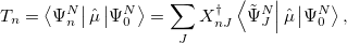
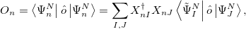
This also allows for the calculation of dipole transition moments via
 |
(6.69) |
as well as excited state properties via
 |
(6.70) |
where  is the property associated with operator
  .
.
Up to now, the exact  -electron ground state has been employed in the derivation of the ADC scheme, thereby resulting in exact excitation energies and exact excited state wave functions. Since the exact ground state is usually not known, a suitable approximation must be used in the derivation of the ISR equations. An obvious choice is the th order Møller-Plesset ground state yielding the th order approximation of the ADC scheme. The appropriate ADC equations have been derived in detail up to third order in Refs. Trofimov:1995,Trofimov:1999,Trofimov:2002. Due to the dependency on the Møller-Plesset ground state the th order ADC scheme should only be applied to molecular systems whose ground state is well described by the respective MP() method.
As in Møller-Plesset perturbation theory, the first ADC scheme which goes beyond the non-correlated wave function methods in Section 6.2 is ADC(2). ADC(2) is available in a strict and an extended variant which are usually referred to as ADC(2)-s and ADC(2)-x, respectively. The strict variant ADC(2)-s scales with the 5th power of the basis set. The quality of ADC(2)-s excitation energies and corresponding excited states is comparable to the quality of those obtained with CIS(D) (Section 6.6) or CC2. More precisely, excited states with mostly single excitation character are well-described by ADC(2)-s, while excited states with double excitation character are usually found to be too high in energy. The ADC(2)-x variant which scales as the sixth power of the basis set improves the treatment of doubly excited states, but at the cost of introducing an imbalance between singly and doubly excited states. As result, the excitation energies of doubly excited states are substantially decreased in ADC(2)-x relative to the states possessing mostly single excitation character with the excitation energies of both types of states exhibiting relatively large errors. Still, ADC(2)-x calculations can be used as a diagnostic tool for the importance doubly excited states in the low-energy region of the spectrum by comparing to ADC(2)-s results. A significantly better description of both singly and doubly excited states is provided by the third order ADC scheme ADC(3). The accuracy of excitation energies obtained with ADC(3) is almost comparable to CC3, but at computational costs that scale with the sixth power of the basis set only [480].
6.8.2 Resolution of the Identity ADC Methods
Similar to MP2 and CIS(D), the ADC equations can be reformulated using the resolution-of-the-identity (RI) approximation. This significantly reduces the cost of the integral transformation and the storage requirements. Although it does not change the overall computational scaling of  for ADC(2)-s or
  for ADC(2)-x with the system size, employing the RI approximation will result in computational speed-up of calculations of larger systems.
The RI approximation can be used with all available ADC methods. It is invoked as soon as an auxiliary basis set is specified using AUX_BASIS.
6.8.3 Spin Opposite Scaling ADC(2) Models
The spin-opposite scaling (SOS) approach originates from MP2 where it was realized that the same spin contributions can be completely neglected, if the opposite spin components are scaled appropriately. In a similar way it is possible to simplify the second order ADC equations by neglecting the same spin contributions in the ADC matrix, while the opposite-spin contributions are scaled with appropriate semi-empirical parameters. [490, 491, 481]
Starting from the SOS-MP2 ground state the same scaling parameter  is introduced into the ADC equations to scale the
  amplitudes. This alone, however, does not result in any computational savings or substantial improvements of the ADC(2) results. In addition, the opposite spin components in the ph/2p2h and 2p2h/ph coupling blocks have to be scaled using a second parameter
  to obtain a useful SOS-ADC(2)-s model. With this model the optimal value of the parameter has been found to be 1.17 for the calculation of singlet excited states.[491]
To extend the SOS approximation to the ADC(2)-x method yet another scaling parameter  for the opposite spin components of the off-diagonal elements in the 2p2h/2p2h block has to be introduced. Here, the optimal values of the scaling parameters have been determined as
  and
and  keeping
  unchanged.[481]
The spin-opposite scaling models can be invoked by setting METHOD to either SOSADC(2) or SOSADC(2)-x. By default, the scaling parameters are chosen as the optimal values reported above, i.e. and  for ADC(2)-s and , , and for ADC(2)-x. However, it is possible to adjust any of the three parameters by setting ADC_C_T, ADC_C_C, or ADC_C_X, respectively.
6.8.4 Core-Excitation ADC Methods
Core-excited electronic states are located in the high energy X-ray region of the spectrum. Thus, to compute core-excited states using standard diagonalization procedures, which usually solve for the energetically lowest-lying excited states first, requires the calculation of a multitude of excited states. This is computationally very expensive and only feasible for calculations on very small molecules and small basis sets.
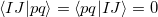
The core-valence separation (CVS) approximation solves the problem by neglecting the couplings between core and valence excited states a priori. [492, 493] Thereby, the ADC matrix acquires a certain block structure which allows to solve only for core-excited states. The application of the CVS approximation is justified, since core and valence excited states are energetically well separated and the coupling between both types of states is very small. To achieve the separation of core and valence excited states the CVS approximation forces the following types of two-electron integrals to zero
 |
|||
 |
(6.71) | ||
 |
where capital letters  refer to core orbitals while lower-case letters
  denote non-core occupied or virtual orbitals.
The core-valence approximation is currently available of ADC models up to third order (including the extended variant). [482, 483, 484] It can be invoked by setting METHOD to the respective ADC model prefixed by CVS. Besides the general ADC related keywords, two additional keywords in the $rem block are necessary to control CVS-ADC calculations:
ADC_CVS = TRUE switches on the CVS-ADC calculation
CC_REST_OCC = n controls the number of core orbitals included in the excitation space. The integer n corresponds to the n energetically lowest core orbitals.
Example: cytosine with the molecular formula C H
H N
N O includes one oxygen atom. To calculate O 1s core-excited states, CC_REST_OCC has to be set to 1, because the 1s orbital of oxygen is the energetically lowest. To obtain the N 1s core excitations, the integer has to be set to 4, because the 1s orbital of the oxygen atom is included as well, since it is energetically below the three 1s orbitals of the nitrogen atoms. Accordingly, to simulate the C 1s XAS spectrum of cytosine, CC_REST_OCC must be set to 8.
To obtain the best agreement with experimental data, one should use the CVS-ADC(2)-x method in combination with at least a diffuse triple- basis set. [482, 483, 484]
6.8.5 Spin-Flip ADC Methods
The spin-flip (SF) method [451, 404, 458, 494] is used for molecular systems with few-reference wave functions like diradicals, bond-breaking, rotations around single bonds, and conical intersections. Starting from a triplet ( ) ground state reference a spin-flip excitation operator
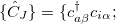

 is introduced, which flipped the spin of one electron while singlet and (
 ) triplet excited target states are yielded. The spin-flip method is implemented for the ADC(2) (strict and extended) and the ADC(3) methods. [494] Note that high-spin () triplet states can be calculated with the SF-ADC method as well using a closed-shell singlet reference state. The number of spin-flip states that shall be calculated is controlled with the $rem variable SF_STATES.
6.8.6 Properties and Visualization
The calculation of excited states using the ADCMAN module yields by default the usual excitation energies and the excitation amplitudes, as well as the transition dipole moments, oscillator strengths, and the norm of the doubles part of the amplitudes (if applicable). In addition, the calculation of excited state properties, like dipole moments, and transition properties between excited states can be requested by setting the $rem variables ADC_PROP_ES and ADC_PROP_ES2ES, respectively. Resonant two-photon absorption cross-sections of the excited states can be computed as well, using either sum-over-states expressions or the matrix inversion technique. The calculation via sum-over-state expressions is automatically activated, if ADC_PROP_ES2ES is set. The accuracy of the results, however, strongly depends on the number of states which are included in the summation, i.e. the number of states computed. At least, 20-30 excited states (per irreducible representation) are required to yield useful results for the two-photon absorption cross-sections. Alternatively, the resonant two-photon absorption cross-sections can be calculated by setting ADC_PROP_TPA to TRUE. In this case, the computation of a large number of excited states is avoided and there is no dependence on the number of excited states. Instead, an additional linear matrix equation has to be solved for every excited state for which the two-photon absorption cross-section is computed. Thus, the obtained resonant two-photon absorption cross-sections are usually more reliable.
Furthermore, the ADCMAN module allows for the detailed analysis of the excited states and export of various types of excited state related orbitals and densities. This can be activated by setting the keyword STATE_ANALYSIS. Details on the available analyses and export options can be found in section 10.2.7.
6.8.7 Excited States in Solution with ADC/SS-PCM
ADCMAN is interfaced to the versatile polarizable-continuum model (PCM) implemented in Q-Chem (Section 11.2.2), which enables a calculation and analysis of excited-state wave functions in solution. The interface follows the state-specific approach and supports a self-consistent equilibration of the solvent-field for long-lived excited states commonly referred to as equilibrium solvation, as well as the calculation of perturbative corrections for vertical transitions, known as non-equilibrium solvation (see also section 11.2.2.3). Combining both approaches, virtually all photochemically relevant processes can be modeled, including ground- and excited-state absorption, fluorescence, phosphorescence, as well as photochemical reactivity. Requiring only the electron-densities of ground- and excited states of the solute as well as and the dielectric constant and refractive index of the solvent, ADC/SS-PCM is straightforward to set up and works with all orders and variants of ADC for which densities are available via the ISR. This includes all levels of canonical ADC, SOS-ADC, SF-ADC for electronically complicated situations, as well as CVS-ADC for the description of core-excited states and the respective resolution of the identity variants. Solvent-relaxed wave functions can be visualized and analyzed using the interface to libwfa.
The theory in this section is limited to a brief, qualitative introduction with only the most important equations, leaving out major aspects such as the polarization work. For a comprehensive, formal introduction to the theory please be referred to Refs. Mewes:2015a and Mewes:2017 as well as sections 11.2.2 and11.2.2.3.
6.8.7.1 Modeling the Absorption Spectrum in Solution
(A) Theory
Let us begin with a brief review of the theoretical and technical aspects of the calculation of absorption spectra in solution. For this purpose, one would typically employ the perturbative, state-specific approach in combination with an ADC of second or third order. The first step is a self-consistent reaction field calculation [SCRF, Hartree-Fock with a PCM, Eq. eq:ADC_SCRF].
 |
(6.72) |
The PCM is formally represented by the reaction- or solvent-field operator  . In practice, is a set of point charges placed on the molecular surface, which are optimized together with the orbitals during the SCF procedure. Note that since accounts for the self-induced polarization of the solute, it depends on solute’s wave function, which will in the following be indicated in the subscript
  .
.
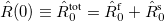
After the SCRF is converged, the final surface-charges and the respective operator can, according to the Franck-Condon principle, be separated into a “slow” solvent-nuclei related ( ) and “fast”, solvent-electron related (
 ) component (eq. eq:ADC_R_sep), and are stored on disk.
 |
(6.73) |
 |
(6.74) |
The “polarized” MOs resulting from the SCRF step are subjected to ordinary MP/ADC calculations, which yield energies and densities for the correlated ground- and excited-states. However, since the MOs contain the interaction with the “frozen” solvent-polarization of the SCF ground-state density ( , i.e., both components), the resulting excitation energies violate the Franck-Condon principle, which requires the solvent-electrons (fast component of the polarization) to be relaxed. Furthermore, the solvent-field is obtained for the SCF density, which more often than not provides a poor description of the electrostatic nature of the solute and may in turn lead to systematic errors in the excitation energies.
To account for the relaxation of the solvent-electrons, the perturbative ansatz shown in eq. eq:ADC_ptSS is employed, in which the fast component of the ground-state solvent field  is replaced by the respective quantity computed for the excited-state density
  . In this framework, the excitation energy of an excited state
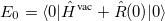
  computed with the polarized MOs can be identified as the zeroth-order energy (eq. eq:ADC_PT_zeroth), while the first-order term becomes the difference between the interaction of the zeroth-order excited-state density with the fast component of the ground- and excited-state solvent fields given in eq. eq:ADC_PT_first.
 |
(6.75) |
 |
 |
 |
(6.76) | ||
 |
|
 |
(6.77) | ||
 |
|
 |
(6.78) |
After the ADC iterations have converged, is computed from the respective excited-state density and read from disk to form the first-order correction. Adding this so-called ptSS-term to the zeroth order energy, one arrives at the vertical excitation energy in the non-equilibrium limit  . Since the ptSS-term accounts for the response of the electron density of the implicit solvent molecules to excitation of the solute, its always a negative and lowers the excitation energy.
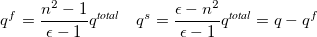
To eliminate problems resulting from the poor description of the ground-state solvent-field at the SCF/HF level of theory, we use an additive correction that is based on the MP2 ground-state density. In a nutshell, it replaces the interaction between the potential of the difference density of the excited state  with the SCF solvent-field
  by the respective interaction with the MP solvent field
  :
:
 |
 |
(6.79) | ||
 |
 |
(6.80) |
We will in the following refer to this as “perturbative, density-based” (PTD) correction and denote the respective approach as ptSS(PTD). Accordingly, the non-PTD corrected results will be denoted ptSS(PTE).
In addition to the ptSS-PCM discussed above, a perturbative variant of the so-called linear response corrections (termed ptLR presented in Ref. Mewes:2015a) is also available. In contrast to the ptSS approach, the ptLR corrections depend on the transition rather than the state (difference) densities. Although the ptLR corrections are always computed and printed, we discourage their use with the correlated ADC variants (2 and higher), for which the ptSS approach is better suited. The ptSS and ptLR approaches are also available for TDDFT as described in Section 11.2.2.3.
A detailed, comprehensive introduction to the theory and implementation, as well as extensive benchmark data for the non-equilibrium formalism in combination with all orders of ADC can be found in Ref. Mewes:2015a.
(B) Usage
The calculation of vertical-transition energies in with the ptSS-PCM approach is fairly straightforward. For any ADC calculation, you just need to activate the PCM by specifying SOLVENT_METHOD PCM in the $rem block and input the solvent parameters, i.e., dielectric constant  (DIELECTRIC) and squared refractive index (DIELECTRIC_INFI) in the $solvent block. Note that the PCM does not support symmetry.
In the output of a ptSS-PCM calculation for all correlated ADC variants, three values are given for the total and transition energies:
Zeroth-order results (direct outcome of the MP/ADC calculation, used for ordering)
First-order results (incl. non-equilibrium effects via ptSS-term)
Corrected first-order results (incl. ptSS-term and the PTD correction)
Note: The zeroth-order results are by no means identical to the gas-phase excitation energies, and in turn the ptSS-term is not the solvatochromic shift.
We recommend to use the corrected first-order results since the PTD correction generally improves the results, in particular if large differences between the SCF and MP2 electrostatics exist. In most cases, the ptSS(PTD) approach is a very good approximation to the fully consistent, but more expensive PTED scheme, in which the solvent field is made self-consistent with the MP2 density (see next section for the PTED scheme and sample-jobs for a comparison of the two). Oscillator strengths are computed using the ptSS(PTD) energies, which are, in general, the most accurate. The PTD* approach includes an empirical scaling of the PTD correction was derived from the solvatochromic-shifts of a series of nitro-aromatics, for which this approach may be superior. Apart from the total and transition energies, all contributing terms (ptSS, PTD etc.) are given separately. A more verbose output detailing all the integrals contributing to the 1st order corrections can be obtained by increasing PCM_PRINT to 1.
(C) Tips and Tricks
To model the absorption spectrum in polar solvents, it is advisable to use a structure optimized in the presence of a PCM since the influence can be quite significant.
It should also be taken into account that a PCM lacks at the description of explicit interactions like e.g. hydrogen bonds. If fairly strong h-bond donors/acceptors are present and a protic/Lewis-basic solvent is to be modeled, consider adding a few (one or maximum two per donor/acceptor site) explicit solvent molecules (and optimize them together with the molecule in the presence of a PCM). A systematic investigation of this aspect for two representative examples can be found in Ref. Mewes:2015a.
If large differences between the HF and MP description of the molecule exist (PTD terms  eV), it is advisable to employ the iterative ptSS(PTED) scheme described in the next section. Due to the inverse nature of the systematic errors of ADC(2) and ADC(3), the best guess for the excitation energy in solution is usually the average of both values.
For the PCM, we recommend the formally exact and slightly more expensive integral-equation formalism (IEF)-PCM variant (THEORY to IEFPCM in the $pcm block) in place of the approximate C-PCM, and otherwise default parameters.
6.8.7.2 Modeling Emission, Excited-State Absorption and Photochemical Reactivity
(A) Theory
To model emission/absorption of solvent-equilibrated excited states and/or to investigate their photochemical reactivity, both components of the polarization have to be relaxed with respect to the desired state. This becomes evident considering that a full solvent-field equilibration (i.e., including the nuclear component) is essentially a geometry optimization for the implicit solvent, and should thus be employed whenever the geometry of the solute is optimized for the desired excited state. The Hamiltonian for a solvent-equilibrated state  simply reads
 |
(6.81) |
Since the interaction with solvent-field is contained in the MOs, the solvent-field of the desired excited state has to be employed already in SCF step of the calculation. This means that a guess (e.g. from a previous calculation) of the solvent-field has to be used for the first SCF calculation. The resulting MOs are subjected to an ADC calculation, yielding a excited-state density, for which a new solvent field is computed and employed in the SCF of the next iteration. This is repeated until the solvent field (charges) and energies are converged, yielding the total energy and wave function of the solvent-equilibrated excited state . However, as the name already suggest, this state-specific approach yields a meaningful energy only for the solvent-equilibrated reference state . All other states have to be treated in the non-equilibrium limit and subjected to the formalism presented in the previous section to be consistent with the Franck-Condon principle. The respective generalization of the perturbative ansatz for the Hamiltonian for the  out-of-equilibrium state (e.g. the ground or any other excited state) in the field of the equilibrated state reads as
 |
(6.82) |
which can be solved using the procedure introduced in the previous section.
While most of the technical aspects concerning the application of the model will be covered in the following, we highly recommend to read at least the formalism and implementation section of Ref. Mewes:2017 before using the model.
(B) Usage
The main switch for the equilibrium solvation SS-PCM is EQSOLV in the $pcm block (SOLVENT_METHOD = PCM has to be set as well). Setting it to TRUE will cause one SCF+ADC calculation to be carried out employing the solvent-field that is found on disk, while any integer  triggers the automatic solvent-field optimization and is interpreted as the maximum number of steps. We recommend to use EQSOLV = 15.
Note: A SS-PCM calculation always requires a preceding converged ptSS-PCM calculation (i.e., EQSOLV = FALSE) for the desired state to provide a guess for the initial solvent-field, or it will crash.
Consequently, the SS-PCM calculation is always the second (or third...) step of a multi-step job. To create the input-file for a multi step job, just add "@@@" at the end of the input for the first job and append the input for the second job. See also section 3.6. Since the reaction-field is stored in the basis of the molecular-surface elements, the geometry of the molecule as well as parameters that affect construction and discretization of the molecular cavity can not be changed between jobs. This, however, is not enforced.
The state for which the solvent field should to be optimized is specified with the variable EQSTATE in the $pcm block. A value of 0 refers to the MP ground-state (for PTED calculations), 1 selects the energetically lowest excited state, 2 the second lowest, and so on. The solvent-field can in principle be optimized for any singlet, triplet or spin-flip excited state. However, only the desired class of states should be requested, i.e., either EE_SINGLETS or EE_TRIPLETS for singlet references, and either EE_STATES or SF_STATES for triplet references. To compute, e.g., the phosphorescence energy, only triplet states should be requested and EQSTATE would typically be set to the lowest excited state.
Note: Computing multiple different classes of excited states during the iterations will confuse the state-counting logic of the program.
Convergence is controlled by EQS_CONV. Criteria are the SCF energy as well as the RMSD, MAD and largest single difference of the surface-charges. The convergence should not need to be modified. It is per default derived from the SCF convergence parameter (SCF_CONVERGENCE ). The default value of 4 (since SCF_CONVERGENCE is 8 for ADC calculations) corresponds to an maximum energy change of
  meV and will yield converged total energies for all states. Excitation energies and in particular the total energy of the reference state converge somewhat faster than the SCF energy, and a value of 3 may save some time for the computation e.g. the emission energy of large solutes.
The self-consistent SS-PCM can also be used to compute a fully consistent solvent-field for the MP2 ground state by setting EQSTATE to 0. This is known as ptSS(PTED) approach and can improve vertical excitation energies if there are large differences between the electrostatic properties of the SCF and MP ground states (large PTD corrections). In most cases, however, the non-iterative PTD approach is a very good approximation to the PTED approach (see the sample jobs below).
The program possesses limited intelligence in detecting the type of the calculation (PTED or EQS/SS-PCM) as well as the target state of the solvent-field equilibration and will assemble and designate the ptSS corrections, total energies and transition energies accordingly. This logic can be confused if multiple classes of states (e.g. singlet and triplets) are computed simultaneously during the iterations, and/or if the ordering of the states changes. Computing singlet and triplet states together in a final job for a previously converged solvent-field should yield a correct output, but will confuse the state counting in any following steps. The output of a PTED calculation is essentially identical to that of the other ptSS-schemes.
In the “HF/MP2/MP3 Summary” section, zeroth (without ptSS) and first (with ptSS) order total energies of the respective ground-state in the solvent-field of the target state are given along with the ptSS term for a vertical transition from the equilibrated state (emission). Note that to obtain the MP3 ground state energy during an ADC(3)/EQS calculation, the ptSS term has to be added manually (it is printed in the MP2 Summary) and moreover, that the HF-dipole moment is currently incorrect (known bug). A correct HF dipole can be found at the end of the output file.
In the “Excited-State Summary” section the reference state is distinguished from the out-of-equilibrium states. Respective total and transition energies are given along with the non-equilibrium corrections, transition moments and some remarks. Note that for emission, in contrast to absorption, the ptSS term increases the transition energy as it lowers the energy of the out-of-equilibrium ground state. The so-called "self-ptSS term" is a perturbative estimate of how much the solvent field of this state is off from its equilibrium. Although the line in the output changes depending on the value (from "not converged" to "reasonably converged" to "converged") it is not used in the actual convergence check. Note that the self-ptSS term is computed with (dielectric_infi) and not , as it probably should be. The self-ptSS term may be used to judge how well a solvent-field computed with a different methodology (basis, ADC order/variant) fits. In such a case, values  eV signal a reasonable agreement.
To calculate inter-state transition moments for excited-state absorption, the variable ADC_PROP_ES2ES has to be set to TRUE. Unfortunately, transition energies have to be computed manually from the (first-order) total energies given in the excited-state summary, since the transition energies given along with the state-to-state transition moments following the excite-state summary are incorrect (missing non-equilibrium terms).
The progress of the solvent-field iteration and their convergence is reported following the “Excited-State Summary”.
(C) Tips and Tricks
To compute fluorescence and phosphorescence energies, solute geometry AND solvent-field should both be optimized for the suspected emitting state. Since hardly any programs can perform excited-state optimizations with the SS-PCM solvent models, you will probably have to use gas-phase geometries. In our experience, the errors introduced by this approximation are small to negligible (typically  eV) in non-polar solvents, but can become significant in polar solvents, in particular for polar charge-transfer states.
Concerning the predicted emission energies, we found that ADC(2)/SS-PCM typically over-stabilizes CT states, yielding emission energies that are too low. SOS-ADC(2) can improve this error, but does not eliminate it. In general, while emission energies are more accurate with (SOS-)ADC(2)/SS-PCM than with ADC(3)/SS-PCM, the latter affords better relative state energies (see Ref. Mewes:2017).
Keep in mind that the solute-solvent interaction of polar solvents with polar (e.g. charge-transfer) states can become quite large (multiple eV), and may thus affect the ordering and nature of the excited states. It should be carefully checked if the character and/or energetic ordering of the states changes during the procedure. This applies in particular to any equilibration of the solvent field for higher lying excited states (e.g.  or
or  ). In one example, however, even the solvent-field equilibration for a weakly polar
  in a polar solvent eventually caused a more polar state (former ) to become the lowest state during the iterations. If the excited-states swap during the procedure, find out in which step the swap occurred and do only so many iterations (i.e., set EQSOLV accordingly). In a following job, adjust the variable EQSTATE and continue the iterations. If states start to mix when they get close, it might help to use an artificially large dielectric constant in a first job to induce the change in state ordering and continue with the desired dielectric constant in the second job.
If performance is critical, the calculations may be accelerated by lowering the ADC convergence during the solvent-field iterations (set ADC_DAVIDSON_CONVERGENCE = 5). The number of iterations may be reduced by first converging the solvent-field with a smaller basis/at a lower level of ADC followed by another job with the full basis/level of ADC. However, in our experience ADC(2) and ADC(3) solvent-fields for the same state differ quite significantly and the approach probably does not help much. In contrast, the solvent-field computed with a smaller basis (e.g. SVP) is often a good approximation for that computed with a larger basis (e.g. def2-TZVP, see examples), such this may actually help. It is in general advisable to compute just as many states as is necessary during the solvent-field iterations and include higher lying excited states and triplets in the final job. In ADC(2) calculations for large systems, one should always employ the resolution-of-the-identity approximation.
To save time in PTED jobs, it is suggested to disable the computation of excited states during the solvent-field iterations of a PTED job by setting EE_SINGLETS (and/or EE_TRIPLETS/ EE_STATES) to 0 and compute the excited-states in a final job once the reaction field is converged.
For more tips and examples see the sample jobs.
6.8.8 Frozen-Density Embedding: FDE-ADC methods
FDE-ADC [497] represents a method to include interactions between an embedded species and its environment into an ADC() calculation based on Frozen Density Embedding Theory (FDET) [498, 499]. FDE-ADC supports ADC and CVS-ADC methods of orders 2s,2x and 3 and regular ADC job control keywords also apply.
The FDE-ADC method starts with generating an embedding potential using a MP() density for the embedded system (A) and a DFT or HF density for the environment (B). A Hartree-Fock calculation is then carried out during which the embedding potential is added to the Fock operator. The embedded Hartree-Fock orbitals act as an input for the subsequent ADC calculation which yields the embedded properties (vertical excitation energies, oscillator strengths, etc.). Further information on the FDE-ADC method and FDE-ADC job control are described in Section 11.7.1.
6.8.9 ADC Job Control
For an ADC calculation it is important to ensure that there are sufficient resources available for the necessary integral calculations and transformations. These resources are controlled using the $rem variables MEM_STATIC and MEM_TOTAL. The memory used by ADC is currently 95% of the difference MEM_TOTAL - MEM_STATIC.
An ADC calculation is requested by setting the $rem variable METHOD to the respective ADC variant. Furthermore, the number of excited states to be calculated has to be specified using one of the $rem variables EE_STATES, EE_SINGLETS, or EE_TRIPLETS. The former variable should be used for open-shell or unrestricted closed-shell calculations, while the latter two variables are intended for restricted closed-shell calculations. Even though not recommended, it is possible to use EE_STATES in a restricted calculation which translates into EE_SINGLETS, if neither EE_SINGLETS nor EE_TRIPLETS is set. Similarly, the use EE_SINGLETS in an unrestricted calculation will translate into EE_STATES, if the latter is not set as well.
All $rem variables to set the number of excited states accept either an integer number or a vector of integer numbers. A single number specifies that the same number of excited states are calculated for every irreducible representation the point group of the molecular system possesses (molecules without symmetry are treated as  symmetric). In contrast, a vector of numbers determines the number of states for each irreducible representation explicitly. Thus, the length of the vector always has to match the number of irreducible representations. Hereby, the excited states are labeled according to the irreducible representation of the electronic transition which might be different from the irreducible representation of the excited state wave function. Users can choose to calculate any molecule as symmetric by setting CC_SYMMETRY = FALSE.
METHOD
Controls the order in perturbation theory of ADC.
TYPE:
STRING
DEFAULT:
None
OPTIONS:
ADC(1)
Perform ADC(1) calculation.
ADC(2)
Perform ADC(2)-s calculation.
ADC(2)-x
Perform ADC(2)-x calculation.
ADC(3)
Perform ADC(3) calculation.
SOS-ADC(2)
Perform spin-opposite scaled ADC(2)-s calculation.
SOS-ADC(2)-x
Perform spin-opposite scaled ADC(2)-x calculation.
CVS-ADC(1)
Perform ADC(1) calculation of core excitations.
CVS-ADC(2)
Perform ADC(2)-s calculation of core excitations.
CVS-ADC(2)-x
Perform ADC(2)-x calculation of core excitations.
RECOMMENDATION:
None
EE_STATES
Controls the number of excited states to calculate.
TYPE:
INTEGER/ARRAY
DEFAULT:
0
Do not perform an ADC calculation
OPTIONS:

Number of states to calculate for each irrep or
![$[n_1, n_2, ...]$](images/img-1056.png)
Compute
states for the first irrep,
states for the second irrep, ...
RECOMMENDATION:
Use this variable to define the number of excited states in case of unrestricted or open-shell calculations. In restricted calculations it can also be used, if neither EE_SINGLETS nor EE_TRIPLETS is given. Then, it has the same effect as setting EE_SINGLETS.
EE_SINGLETS
Controls the number of singlet excited states to calculate.
TYPE:
INTEGER/ARRAY
DEFAULT:
0
Do not perform an ADC calculation of singlet excited states
OPTIONS:
Number of singlet states to calculate for each irrep or
Compute
RECOMMENDATION:
Use this variable to define the number of excited states in case of restricted calculations of singlet states. In unrestricted calculations it can also be used, if EE_STATES not set. Then, it has the same effect as setting EE_STATES.
EE_TRIPLETS
Controls the number of triplet excited states to calculate.
TYPE:
INTEGER/INTEGER ARRAY
DEFAULT:
0
Do not perform an ADC calculation of triplet excited states
OPTIONS:
Number of triplet states to calculate for each irrep or
Compute
RECOMMENDATION:
Use this variable to define the number of excited states in case of restricted calculations of triplet states.
CC_SYMMETRY
Activates point-group symmetry in the ADC calculation.
TYPE:
LOGICAL
DEFAULT:
TRUE
If the system possesses any point-group symmetry.
OPTIONS:
TRUE
Employ point-group symmetry
FALSE
Do not use point-group symmetry
RECOMMENDATION:
None
ADC_PROP_ES
Controls the calculation of excited state properties (currently only dipole moments).
TYPE:
LOGICAL
DEFAULT:
FALSE
OPTIONS:
TRUE
Calculate excited state properties.
FALSE
Do not compute state properties.
RECOMMENDATION:
Set to TRUE, if properties are required.
ADC_PROP_ES2ES
Controls the calculation of transition properties between excited states (currently only transition dipole moments and oscillator strengths), as well as the computation of two-photon absorption cross-sections of excited states using the sum-over-states expression.
TYPE:
LOGICAL
DEFAULT:
FALSE
OPTIONS:
TRUE
Calculate state-to-state transition properties.
FALSE
Do not compute transition properties between excited states.
RECOMMENDATION:
Set to TRUE, if state-to-state properties or sum-over-states two-photon absorption cross-sections are required.
ADC_PROP_TPA
Controls the calculation of two-photon absorption cross-sections of excited states using matrix inversion techniques.
TYPE:
LOGICAL
DEFAULT:
FALSE
OPTIONS:
TRUE
Calculate two-photon absorption cross-sections.
FALSE
Do not compute two-photon absorption cross-sections.
RECOMMENDATION:
Set to TRUE, if to obtain two-photon absorption cross-sections.
STATE_ANALYSIS
Controls the analysis and export of excited state densities and orbitals (see 10.2.7 for details).
TYPE:
LOGICAL
DEFAULT:
FALSE
OPTIONS:
TRUE
Perform excited state analyses.
FALSE
No excited state analyses or export will be performed.
RECOMMENDATION:
Set to TRUE, if detailed analysis of the excited states is required or if density or orbital plots are needed.
ADC_C_T
Set the spin-opposite scaling parameter
.
TYPE:
INTEGER
DEFAULT:
1300
Optimized value
.
OPTIONS:
Corresponding to

RECOMMENDATION:
Use the default.
ADC_C_C
Set the spin-opposite scaling parameter
TYPE:
INTEGER
DEFAULT:
1170
Optimized value
1000
OPTIONS:
Corresponding to
RECOMMENDATION:
Use the default.
ADC_C_X
Set the spin-opposite scaling parameter
TYPE:
INTEGER
DEFAULT:
1300
Optimized value
for ADC(2)-x.
OPTIONS:
Corresponding to
RECOMMENDATION:
Use the default.
ADC_NGUESS_SINGLES
Controls the number of excited state guess vectors which are single excitations. If the number of requested excited states exceeds the total number of guess vectors (singles and doubles), this parameter is automatically adjusted, so that the number of guess vectors matches the number of requested excited states.
TYPE:
INTEGER
DEFAULT:
Equals to the number of excited states requested.
OPTIONS:
User-defined integer.
RECOMMENDATION:
ADC_NGUESS_DOUBLES
Controls the number of excited state guess vectors which are double excitations.
TYPE:
INTEGER
DEFAULT:
0
OPTIONS:
User-defined integer.
RECOMMENDATION:
ADC_DO_DIIS
Activates the use of the DIIS algorithm for the calculation of ADC(2) excited states.
TYPE:
LOGICAL
DEFAULT:
FALSE
OPTIONS:
TRUE
Use DIIS algorithm.
FALSE
Do diagonalization using Davidson algorithm.
RECOMMENDATION:
None.
ADC_DIIS_START
Controls the iteration step at which DIIS is turned on.
TYPE:
INTEGER
DEFAULT:
1
OPTIONS:
User-defined integer.
RECOMMENDATION:
Set to a large number to switch off DIIS steps.
ADC_DIIS_SIZE
Controls the size of the DIIS subspace.
TYPE:
INTEGER
DEFAULT:
7
OPTIONS:
User-defined integer
RECOMMENDATION:
None
ADC_DIIS_MAXITER
Controls the maximum number of DIIS iterations.
TYPE:
INTEGER
DEFAULT:
50
OPTIONS:
User-defined integer.
RECOMMENDATION:
Increase in case of slow convergence.
ADC_DIIS_ECONV
Controls the convergence criterion for the excited state energy during DIIS.
TYPE:
INTEGER
DEFAULT:
6
Corresponding to

OPTIONS:
Corresponding to

RECOMMENDATION:
None
ADC_DIIS_RCONV
Convergence criterion for the residual vector norm of the excited state during DIIS.
TYPE:
INTEGER
DEFAULT:
6
Corresponding to
OPTIONS:
Corresponding to
RECOMMENDATION:
None
ADC_DAVIDSON_MAXSUBSPACE
Controls the maximum subspace size for the Davidson procedure.
TYPE:
INTEGER
DEFAULT:
the number of excited states to be calculated.
OPTIONS:
User-defined integer.
RECOMMENDATION:
Should be at least
the number of excited states to calculate. The larger the value the more disk space is required.
ADC_DAVIDSON_MAXITER
Controls the maximum number of iterations of the Davidson procedure.
TYPE:
INTEGER
DEFAULT:
60
OPTIONS:
Number of iterations
RECOMMENDATION:
Use the default unless convergence problems are encountered.
ADC_DAVIDSON_CONV
Controls the convergence criterion of the Davidson procedure.
TYPE:
INTEGER
DEFAULT:

Corresponding to
OPTIONS:

Corresponding to
RECOMMENDATION:
Use the default unless higher accuracy is required or convergence problems are encountered.
ADC_DAVIDSON_THRESH
Controls the threshold for the norm of expansion vectors to be added during the Davidson procedure.
TYPE:
INTEGER
DEFAULT:
Twice the value of ADC_DAVIDSON_CONV, but at maximum
.
OPTIONS:

Corresponding to
RECOMMENDATION:
Use the default unless convergence problems are encountered. The threshold value
ADC_PRINT
Controls the amount of printing during an ADC calculation.
TYPE:
INTEGER
DEFAULT:
1
Basic status information and results are printed.
OPTIONS:
0
Quiet: almost only results are printed.
1
Normal: basic status information and results are printed.
2
Debug: more status information, extended information on timings.
...
RECOMMENDATION:
Use the default.
ADC_CVS
Activates the use of the CVS approximation for the calculation of CVS-ADC core-excited states.
TYPE:
LOGICAL
DEFAULT:
FALSE
OPTIONS:
TRUE
Activates the CVS approximation.
FALSE
Do not compute core-excited states using the CVS approximation.
RECOMMENDATION:
Set to TRUE, if to obtain core-excited states for the simulation of X-ray absorption spectra. In the case of TRUE, the $rem variable CC_REST_OCC has to be defined as well.
CC_REST_OCC
Sets the number of restricted occupied orbitals including active core occupied orbitals.
TYPE:
INTEGER
DEFAULT:
0
OPTIONS:
Restrict
RECOMMENDATION:
Example: cytosine with the molecular formula C
SF_STATES
Controls the number of excited spin-flip states to calculate.
TYPE:
INTEGER
DEFAULT:
0
Do not perform a SF-ADC calculation
OPTIONS:
Number of states to calculate for each irrep or
Compute
RECOMMENDATION:
Use this variable to define the number of excited states in the case of a spin-flip calculation. SF-ADC is available for ADC(2)-s, ADC(2)-x and ADC(3).
Keywords for SS-PCM control in $pcm:
EQSOLV
Main switch of the self-consistent SS-PCM procedure.
INPUT SECTION: $pcm
TYPE:
INTEGER
DEFAULT:
0
OPTIONS:
0
No self-consistent SS-PCM.
1
Single SS-PCM calculation (SCF+ADC) with the solvent-field found on disk.
1
Do a maximum of
RECOMMENDATION:
We recommend to use 15 steps max. Typical convergence is 3-5 steps. In difficult cases 6-12. If the solvent-field iteration do not converge in 15 steps, something is wrong.
Also make sure that a solvent-field has been stored on disk by a previous job.
EQSTATE
Specifies the state for which the solvent-field is to be optimized.
INPUT SECTION: $pcm
TYPE:
INTEGER
DEFAULT:
0
OPTIONS:
0
MP2 ground state (for PTED approach)
1
energetically lowest excited state
2
2nd lowest excited state
...
RECOMMENDATION:
The program will blindly select the state by its energetic position shown in the “Exited-State Summary” part in the output file. A maximum of 99 states can be stored and selected.
EQS_CONV
Controls the convergence of the solvent-field iterations by setting the convergence criteria (a mixture of SCF energy and charge-vector). SCF energy criterion computes as
eH
INPUT SECTION: $pcm
TYPE:
INTEGER
DEFAULT:
SCF_CONVERGENCE

OPTIONS:
3
May be sufficient for emission energies
4
Assured converged total energies (2.7 meV).
5
Really tight
RECOMMENDATION:
Use the default.
6.8.10 Examples
Example 6.178 Q-Chem input for an ADC(2)-s calculation of singlet exited states of methane with D2 symmetry. In total six excited states are requested corresponding to four (two) electronic transitions with irreducible representation  (
( ).
).
$molecule
   0 1
   C
   H   1 r0
   H   1 r0   2  d0
   H   1 r0   2  d0   3  d1
   H   1 r0   2  d0   4  d1

   r0 = 1.085
   d0 = 109.4712206
   d1 = 120.0
$end

$rem
   METHOD              adc(2)
   BASIS               6-31g(d,p)
   MEM_TOTAL           4000
   MEM_STATIC          100
   EE_SINGLETS         [0,4,2,0]
$end
Example 6.179 Q-Chem input for an unrestricted RI-ADC(2)-s calculation with symmetry using DIIS. In addition, excited state properties and state-to-state properties are computed.
$molecule
   0 2
   C    0.0    0.0   -0.630969
   N    0.0    0.0    0.540831
$end

$rem
   METHOD           adc(2)
   BASIS            aug-cc-pVDZ
   AUX_BASIS        rimp2-aug-cc-pVDZ
   MEM_TOTAL        4000
   MEM_STATIC       100
   CC_SYMMETRY      false
   EE_STATES        6
   ADC_DO_DIIS      true
   ADC_PROP_ES      true
   ADC_PROP_ES2ES   true
   ADC_PROP_TPA     true
$end
Example 6.180 Q-Chem input for a restricted CVS-ADC(2)-x calculation with symmetry using 4 parallel CPU cores. In this case, the 10 lowest nitrogen K-shell singlet excitations are computed.
$molecule
   0 1
   C    -5.17920    2.21618    0.01098
   C    -3.85603    2.79078    0.05749
   N    -2.74877    2.08372    0.05569
   C    -5.23385    0.85443   -0.04040
   C    -2.78766    0.70838    0.01226
   N    -4.08565    0.13372   -0.03930
   N    -3.73433    4.14564    0.16144
   O    -1.81716   -0.02560    0.00909
   H    -4.50497    4.74117   -0.12037
   H    -2.79158    4.50980    0.04490
   H    -4.10443   -0.88340   -0.07575
   H    -6.08637    2.82445    0.02474
   H    -6.17341    0.29221   -0.07941
$end

$rem
   METHOD                      cvs-adc(2)-x
   EE_SINGLETS                 10
   ADC_DAVIDSON_MAXSUBSPACE    60
   MEM_TOTAL                   10000
   MEM_STATIC                  1000
   THREADS                     4
   CC_SYMMETRY                 false
   BASIS                       6-31G*
   ADC_DAVIDSON_THRESH         8
   SYMMETRY                    false
   ADC_DAVIDSON_MAXITER        900
   ADC_CVS                     true
   CC_REST_OCC                 4
$end
Example 6.181 Q-Chem input for a restricted SF-ADC(2)-s calculation of the first three spin-flip target states of cyclobutadiene without point group symmetry.
$molecule
   0 3
   C     0.000000     0.000000     0.000000
   C     1.439000     0.000000     0.000000
   C     1.439000     0.000000     1.439000
   C     0.000000     0.000000     1.439000
   H    -0.758726     0.000000    -0.758726
   H     2.197726     0.000000    -0.758726
   H     2.197726     0.000000     2.197726
   H    -0.758726     0.000000     2.197726
$end

$rem
   METHOD          adc(2)
   MEM_TOTAL       15000
   MEM_STATIC      1000
   CC_SYMMETRY     false
   BASIS           3-21G
   SF_STATES       3
$end
Example 6.182 Q-Chem input for a restricted ADC(2)-x calculation of water with  symmetry. Four singlet A" excited states and two triplet A’ excited states are requested. For the first two states (1
 A" and 1
 A’) the transition densities as well as the attachment and detachment densities are exported into cube files.
$molecule
   0 1
   O   0.000   0.000   0.000
   H   0.000   0.000   0.950
   H   0.896   0.000  -0.317
$end

$rem
   METHOD            adc(2)-x
   BASIS             6-31g(d,p)
   THREADS           2
   MEM_TOTAL         3000
   MEM_STATIC        100
   EE_SINGLETS       [0,4]
   EE_TRIPLETS       [2,0]
   ADC_PROP_ES       true
   MAKE_CUBE_FILES   true
$end

$plots
Plot transition and a/d densities
   40 -3.0 3.0
   40 -3.0 3.0
   40 -3.0 3.0
   0 0 2 2
   1 2
   1 2
$end
Example 6.183 Q-Chem input for a ADC(2)-s/ptSS-PCM calculation of the five lowest singlet-excited states of N,N-dimethylnitroaniline in diethylether. PCM settings are all default values except THEORY, which is set to IEFPCM instead of the default CPCM.
$rem
   THREADS                4
   METHOD                 adc(2)
   BASIS                  3-21G
   MEM_TOTAL              32000
   MEM_STATIC             2000
   ADC_PROP_ES            true
   ADC_PRINT              1
   EE_SINGLETS            5
   ADC_DAVIDSON_MAXITER   100
   PCM_PRINT              1       !increase print level
   SOLVENT_METHOD         pcm     !invokes PCM solvent model
$end

$pcm
   StateSpecific           Perturb !default for ADC/PCM
   ChargeSeparation        Marcus  !default
   theory                  IEFPCM  !default is CPCM, IEFPCM is more accurate
   method                  ISWIG
   Solver                  Inversion
   Radii                   Bondi
   vdwScale                1.20
$end

$solvent
   dielectric              4.34  !epsilon of Et2O
   dielectric_infi         1.829 !n_square of Et2O
$end

$molecule
   0 1
   C   -4.263068      2.512843      0.025391
   C   -5.030982      1.361365      0.007383
   C   -4.428196      0.076338     -0.021323
   C   -3.009941      0.019036     -0.030206
   C   -2.243560      1.171441     -0.011984
   C   -2.871710      2.416638      0.015684
   H   -4.740854      3.480454      0.047090
   H   -2.502361     -0.932570     -0.052168
   H   -1.166655      1.104642     -0.020011
   H   -6.104933      1.461766      0.015870
   N   -5.178541     -1.053870     -0.039597
   C   -6.632186     -0.969550     -0.034925
   H   -6.998203     -0.462970      0.860349
   H   -7.038179     -1.975370     -0.051945
   H   -7.001616     -0.431420     -0.910237
   C   -4.531894     -2.358860     -0.066222
   H   -3.912683     -2.476270     -0.957890
   H   -5.298508     -3.126680     -0.075403
   H   -3.902757     -2.507480      0.813678
   N   -2.070815      3.621238      0.033076
   O   -0.842606      3.510489      0.025476
   O   -2.648404      4.710370      0.054545
$end
Example 6.184 Q-Chem input for a ADC/SS-PCM EQS solvent-field equilibration for the first excited singlet state of peroxinitrite in water, which provides e.g. the fluorescence energy. After generating a starting point in the first job (using a smaller basis and lower adc convergence criteria), the solvent-field iterations are carried out until convergence in the second job. In the third job, ADC(2) excited states are computed in the converged solvent field that was left on disk by the second Job. In the fourth job, we additionally compute ADC(3) excited states. This mixed approach should in general be used with great caution. If the self-ptSS term of the reference state becomes too large (>0.01 eV) like it is the case here, the fully consistent approach should be used (i.e. also the solvent-field computed at the ADC(3) level). PCM settings are all default values except THEORY, which is set to IEFPCM instead of the default CPCM.
$comment
   ADC(2)/ptSS-PCM to generate starting point for the EqS
   Step in the next Job
$end

$rem
   THREADS             2
   METHOD              adc(2)
   BASIS               3-21G !using a small basis to speed up this step
   MEM_TOTAL           6000
   MEM_STATIC          1000
   EE_SINGLETS         1
   ADC_PROP_ES         true
   ADC_DAVIDSON_CONV   4
   SOLVENT_METHOD      pcm
$end

$solvent !Water
   dielectric       78.4
   dielectric_infi   1.76
$end

$molecule
   -1 1
   N    -0.068642000000     -0.600693000000     -0.723424000000
   O     0.349666000000      0.711166000000      1.187490000000
   O    -0.948593000000      0.200668000000     -0.956940000000
   O     0.659040000000     -0.386002000000      0.402650000000
$end

@@@

$comment
   ADC(2)/ptSS-PCM(EqS) solvent-field equilibration
   for the first excited state
$end

$rem
   THREADS          2
   METHOD           adc(2)
   BASIS            6-31G*
   MEM_TOTAL        6000
   MEM_STATIC       1000
   EE_SINGLETS      2 !compute 2 singlets during the equilibration
   ADC_PROP_ES      true
   SOLVENT_METHOD   pcm !activate PCM
$end

$pcm
   eqsolv      15    !maximum 15 steps, converges after 5
   eqstate     1     !Equilibrate 1st excited state
   eqs_conv    4     !Default convergence
   theory      iefpcm
$end

$solvent
   dielectric       78.4
   dielectric_infi   1.76
$end

$molecule
   read
$end

@@@

$comment
   Compute ADC(2) excited states in the converged solvent field
$end

$rem
   THREADS          2
   METHOD           adc(2)
   BASIS            6-31G*
   MEM_TOTAL        6000
   MEM_STATIC       1000
   EE_SINGLETS      6 !compute 6 singlets
   ADC_PROP_ES      true
   ADC_PROP_ES2ES   true !compute ES 2 ES transition moments for ESA
   SOLVENT_METHOD   pcm
$end

$pcm
   eqsolv   true !only one calculation with converged field
   eqstate  1    !Equilibrate 1st excited state
   theory   iefpcm
$end

$solvent
   dielectric      78.4
   dielectric_infi  1.76
$end

$molecule
   read
$end

@@@

$comment
   We can also compute ADC(3) excited states in the
   converged ADC(2) solvent field and use the self-
   ptSS term as diagnostic.
$end

$rem
   THREADS          2
   METHOD           adc(3)
   BASIS            6-31G*
   MEM_TOTAL        6000
   MEM_STATIC       1000
   EE_SINGLETS      3 !compute 3 singlets
   EE_TRIPLETS      1    !and 1 triplet
   ADC_PROP_ES      true
   SOLVENT_METHOD   pcm
$end

$pcm
   eqsolv   true !only one calculation with converged field
   eqstate  1    !Equilibrate 1st excited state
   theory   iefpcm
$end

$solvent
   dielectric      78.4
   dielectric_infi  1.76
$end

$molecule
   read
$end
Example 6.185 Q-Chem input for a riADC(2)/ptSS-PCM(PTED) calculation for the five lowest excited states of peroxinitrite in water. After generating a starting point in the first job, which also provides the ptSS(PTE) and ptSS(PTD) results for comparison, the solvent-field is equilibrated for the MP density in the second job. During the iterations, the calculation of excited states is disabled to speed up the calculation. In the third job, five excited states are computed at the riADC(2)/ptSS(PTED) level of theory. Although the PTD corrections for this molecule are unusually large, a comparison of the PTE, PTD and PTD* results from the first job with the PTED results from the third job will reveal a reasonable agreement between the fully consistent PTED and the perturbative PTD approaches. In the fourth job, excited states are calculated with a larger basis set. The self-ptSS term of the MP ground state will be quite small, showing that the solvent-field computed with the smaller SVP basis is a good approximation.
$comment
   riADC(2)/ptSS-PCM to generate starting point for
   the PTED iterations in the next Job and provide
   PTE and PTD energies for comparing with PTED
$end

$rem
   THREADS          2
   METHOD           adc(2)
   BASIS            def2-SVP
   AUX_BASIS        rimp2-VDZ
   MEM_TOTAL        6000
   MEM_STATIC       1000
   EE_SINGLETS      5
   ADC_PROP_ES      true
   SOLVENT_METHOD   pcm
$end

$solvent !Water
   dielectric      78.4
   dielectric_infi  1.76
$end

$molecule
   -1 1
   N    -0.068642000000     -0.600693000000     -0.723424000000
   O     0.349666000000      0.711166000000      1.187490000000
   O    -0.948593000000      0.200668000000     -0.956940000000
   O     0.659040000000     -0.386002000000      0.402650000000
$end

@@@

$comment
   riADC(2)/ptSS-PTED solvent-field equilibration for
   the MP ground state. No excited states are computed
$end

$rem
   THREADS          2
   METHOD           adc(2)
   BASIS            def2-SVP
   AUX_BASIS        rimp2-VDZ
   MEM_TOTAL        6000
   MEM_STATIC       1000
   EE_SINGLETS      0 !dont compute ES
   ADC_PROP_ES      true
   SOLVENT_METHOD   pcm !activate PCM
$end

$pcm
   eqsolv     15    !maximum 15 steps
   eqstate    0     !Equilibrate MP ground state
   eqs_conv   5     !higher convergence
   theory     iefpcm
$end

$solvent
   dielectric      78.4
   dielectric_infi  1.76
$end

$molecule
   read
$end

@@@

$comment
   Compute ADC(2)/ptSS-PTED excited states in the
   converged solvent field
$end

$rem
   THREADS          2
   METHOD           adc(2)
   BASIS            def2-SVP
   AUX_BASIS        rimp2-VDZ
   MEM_TOTAL        6000
   MEM_STATIC       1000
   EE_SINGLETS      5 !compute 5 singlets
   ADC_PROP_ES      true
   SOLVENT_METHOD   pcm
$end

$pcm
   eqsolv   true !only one calculation with converged field
   eqstate  0    !Equilibrate MP ground state
   theory   iefpcm
$end

$solvent
   dielectric 78.4
   dielectric_infi 1.76
$end

$molecule
   read
$end

@@@

$comment
   We can also compute the ES in the converged field
   with a larger basis and without RI in the stored
   solvent-field.
$end

$rem
   THREADS         2
   METHOD          adc(2)
   BASIS           def2-TZVP
   MEM_TOTAL       6000
   MEM_STATIC      1000
   EE_SINGLETS     3 !compute 3 singlets
   ADC_PROP_ES     true
   SOLVENT_METHOD  pcm
$end

$pcm
   eqsolv  true !only one calculation with converged field
   eqstate 0  !Equilibrate MP ground state
   theory iefpcm
$end

$solvent
   dielectric 78.4
   dielectric_infi 1.76
$end

$molecule
   read
$end