4.1 Introduction

4.1.1 Overview of Chapter

Theoretical chemical models [8] involve two principal approximations. One must specify the type of atomic orbital basis set used (see Chapters 7 and 8), and one must specify the way in which the instantaneous interactions (or correlations) between electrons are treated. Self-consistent field (SCF) methods are the simplest and most widely used electron correlation treatments, and contain as special cases all Kohn-Sham density functional methods and the Hartree-Fock method. This Chapter summarizes Q-Chem’s SCF capabilities, while the next Chapter discusses more complex (and computationally expensive!) wavefunction-based methods for describing electron correlation. If you are new to quantum chemistry, we recommend that you also purchase an introductory textbook on the physical content and practical performance of standard methods [8, 9, 10].

This Chapter is organized so that the earlier sections provide a mixture of basic theoretical background, and a description of the minimum number of program input options that must be specified to run SCF jobs. Specifically, this includes the sections on:

Hartree-Fock theory
Density functional theory. Note that all basic input options described in the Hartree-Fock also apply to density functional calculations.

Later sections introduce more specialized options that can be consulted as needed:

Large molecules and linear scaling methods. A short overview of the ideas behind methods for very large systems and the options that control them.
Initial guesses for SCF calculations. Changing the default initial guess is sometimes important for SCF calculations that do not converge.
Converging the SCF calculation. This section describes the iterative methods available to control SCF calculations in Q-Chem. Altering the standard options is essential for SCF jobs that have failed to converge with the default options.
Unconventional SCF calculations. Some nonstandard SCF methods with novel physical and mathematical features. Explore further if you are interested!
SCF Metadynamics. This can be used to locate multiple solutions to the SCF equations and help check that your solution is the lowest minimum.

4.1.2 Theoretical Background

In 1926, Schrödinger [11] combined the wave nature of the electron with the statistical knowledge of the electron viz. Heisenberg’s Uncertainty Principle [12] to formulate an eigenvalue equation for the total energy of a molecular system. If we focus on stationary states and ignore the effects of relativity, we have the time-independent, non-relativistic equation

$\begin{equation} \label{eq400} H({\rm {\bf R}},{\rm {\bf r}})\Psi ({\rm {\bf R}},{\rm {\bf r}})=E({\rm {\bf R}})\Psi ({\rm {\bf R}},{\rm {\bf r}}) \end{equation}$

(4.1)

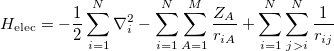
where the coordinates $\ensuremath{\mathbf{R}}$ and $\ensuremath{\mathbf{r}}$ refer to nuclei and electron position vectors respectively and $H$ is the Hamiltonian operator. In atomic units,

$\begin{equation} \label{eq401} H=-\frac{1}{2}\sum \limits _{i=1}^ N {\nabla _ i^2 } -\frac{1}{2}\sum \limits _{A=1}^ M {\frac{1}{M_ A }\nabla _ A^2 } -\sum \limits _{i=1}^ N {\sum \limits _{A=1}^ M {\frac{Z_ A }{r_{iA} }} } +\sum \limits _{i=1}^ N {\sum \limits _{j>i}^ N {\frac{1}{r_{ij} }} } +\sum \limits _{A=1}^ M {\sum \limits _{B>A}^ M {\frac{Z_ A Z_ B }{R_{AB} }} } \end{equation}$

(4.2)

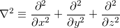
where $\nabla ^{2}$ is the Laplacian operator,

$\begin{equation} \label{eq402} \nabla ^2\equiv \frac{\partial ^2}{\partial x^2}+\frac{\partial ^2}{\partial y^2}+\frac{\partial ^2}{\partial z^2} \end{equation}$

(4.3)

In Eq. eq401, $Z$ is the nuclear charge, $M_{A}$ is the ratio of the mass of nucleus $A$ to the mass of an electron, $R_{AB} = |\ensuremath{\mathbf{R}}_ A - \ensuremath{\mathbf{R}}_ B|$ is the distance between the $A$ th and $B$ th nucleus, $r_{ij} = |\ensuremath{\mathbf{r}}_{i} - \ensuremath{\mathbf{r}}_{j}|$ is the distance between the $i$ th and $j$ th electrons, $r_{iA} = | \ensuremath{\mathbf{r}}_ i - \ensuremath{\mathbf{R}}_ A|$ is the distance between the $i$ th electron and the $A$ th nucleus, $M$ is the number of nuclei and $N$ is the number of electrons. $E$ is an eigenvalue of $H$ , equal to the total energy, and the wave function $\Psi$ , is an eigenfunction of $H$ .

Separating the motions of the electrons from that of the nuclei, an idea originally due to Born and Oppenheimer [13], yields the electronic Hamiltonian operator:

$\begin{equation} \label{eq403} H_{\mathrm{elec}} =-\frac{1}{2}\sum \limits _{i=1}^ N {\nabla _ i^2 } -\sum \limits _{i=1}^ N {\sum \limits _{A=1}^ M {\frac{Z_ A }{r_{iA} }} } +\sum \limits _{i=1}^ N {\sum \limits _{j>i}^ N {\frac{1}{r_{ij} }} } \end{equation}$

(4.4)

The solution of the corresponding electronic Schrödinger equation,

$\begin{equation} \label{eq404} H_{\mathrm{elec}} \Psi _{\mathrm{elec}} =E_{\mathrm{elec}} \Psi _{\mathrm{elec}} \end{equation}$

(4.5)

gives the total electronic energy, $E_{\mathrm{elec}}$ , and electronic wave function, $\Psi _{\mathrm{elec}}$ , which describes the motion of the electrons for a fixed nuclear position. The total energy is obtained by simply adding the nuclear–nuclear repulsion energy [the fifth term in Eq. (4.2)] to the total electronic energy:

$\begin{equation} \label{eq405} E_{\mathrm{tot}} =E_{\mathrm{elec}} +E_{\mathrm{nuc}} \end{equation}$

(4.6)

Solving the eigenvalue problem in Eq. (4.5) yields a set of eigenfunctions ( $\Psi _0$ , $\Psi _1$ , $\Psi _2 \ldots$ ) with corresponding eigenvalues ( $E_0$ , $E_1$ , $E_2\ldots$ ) where $E_0 \le E_1 \le E_2 \le \ldots$ .

Our interest lies in determining the lowest eigenvalue and associated eigenfunction which correspond to the ground state energy and wavefunction of the molecule. However, solving Eq. (4.5) for other than the most trivial systems is extremely difficult and the best we can do in practice is to find approximate solutions.

The first approximation used to solve Eq. (4.5) is that electrons move independently within molecular orbitals (MO), each of which describes the probability distribution of a single electron. Each MO is determined by considering the electron as moving within an average field of all the other electrons. Ensuring that the wavefunction is antisymmetric upon electron interchange, yields the well known Slater-determinant wavefunction [14, 15],

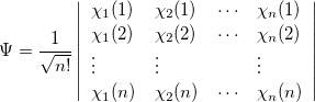$\begin{equation} \label{eq406} \Psi =\frac{1}{\sqrt {n!} }\left| {{\begin{array}{*{20}c} {\chi _1 (1)} \hfill & {\chi { }_2(1)} \hfill & \cdots \hfill & {\chi _ n (1)} \hfill \\ {\chi _1 (2)} \hfill & {\chi _2 (2)} \hfill & \cdots \hfill & {\chi _ n (2)} \hfill \\ \vdots \hfill & \vdots \hfill & \hfill & \vdots \hfill \\ {\chi _1 (n)} \hfill & {\chi _2 (n)} \hfill & \cdots \hfill & {\chi _ n (n)} \hfill \\ \end{array} }} \right| \end{equation}$

(4.7)

where $\chi _ i$ , a spin orbital, is the product of a molecular orbital $\psi _ i$ and a spin function ( $\alpha$ or $\beta$ ).

One obtains the optimum set of MOs by variationally minimizing the energy in what is called a “self-consistent field” or SCF approximation to the many-electron problem. The archetypal SCF method is the Hartree-Fock approximation, but these SCF methods also include Kohn-Sham Density Functional Theories (see Section 4.3). All SCF methods lead to equations of the form

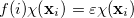$\begin{equation} \label{eq407} f(i)\chi (\ensuremath{\mathbf{x}}_ i )=\varepsilon \chi (\ensuremath{\mathbf{x}}_ i ) \end{equation}$

(4.8)

where the Fock operator $f(i)$ can be written

$\begin{equation} \label{eq408} f(i)=-\frac{1}{2}\nabla _ i^2 +\upsilon ^{\mathrm{eff}}(i) \end{equation}$

(4.9)

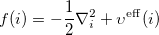
Here $\ensuremath{\mathbf{x}}_ i$ are spin and spatial coordinates of the $i$ th electron, $\chi$ are the spin orbitals and $\upsilon ^{\mathrm{eff}}$ is the effective potential “seen” by the $i$ th electron which depends on the spin orbitals of the other electrons. The nature of the effective potential $\upsilon ^{\mathrm{eff}}$ depends on the SCF methodology and will be elaborated on in further sections.

The second approximation usually introduced when solving Eq. (4.5), is the introduction of an Atomic Orbital (AO) basis. AOs ( $\phi _{\mu }$ ) are usually combined linearly to approximate the true MOs. There are many standardized, atom-centered basis sets and details of these are discussed in Chapter 7.

After eliminating the spin components in Eq. (4.8) and introducing a finite basis,

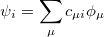$\begin{equation} \label{eq409} \psi _ i =\sum \limits _\mu {c_{\mu i} \phi _\mu } \end{equation}$

(4.10)

Eq. (4.8) reduces to the Roothaan-Hall matrix equation,

$\begin{equation} \label{eq410} {\rm {\bf FC}}=\varepsilon {\rm {\bf SC}} \end{equation}$

(4.11)

where $\ensuremath{\mathbf{F}}$ is the Fock matrix, $\ensuremath{\mathbf{C}}$ is a square matrix of molecular orbital coefficients, $\ensuremath{\mathbf{S}}$ is the overlap matrix with elements

$\begin{equation} \label{eq411} S_{\mu \nu } =\int {\phi _\mu ({\rm {\bf r}})} \phi _\nu ({\rm {\bf r}})d{\rm {\bf r}} \end{equation}$

(4.12)

and ${\varepsilon }$ is a diagonal matrix of the orbital energies. Generalizing to an unrestricted formalism by introducing separate spatial orbitals for $\alpha$ and $\beta$ spin in Eq. (4.7) yields the Pople-Nesbet [16] equations

	$\displaystyle \label{eq412} \ensuremath{\mathbf{F}}^{\alpha } \ensuremath{\mathbf{C}}^{\alpha }$	$\displaystyle =$	$\displaystyle \varepsilon ^{\alpha } \ensuremath{\mathbf{SC}}^{\alpha }\nonumber$
	$\displaystyle \ensuremath{\mathbf{F}}^{\beta } \ensuremath{\mathbf{C}}^{\beta }$	$\displaystyle =$	$\displaystyle \varepsilon ^{\beta } \ensuremath{\mathbf{SC}}^{\beta }$		(4.13)

Solving Eq. (4.11) or Eq. (4.13) yields the restricted or unrestricted finite basis Hartree-Fock approximation. This approximation inherently neglects the instantaneous electron-electron correlations which are averaged out by the SCF procedure, and while the chemistry resulting from HF calculations often offers valuable qualitative insight, quantitative energetics are often poor. In principle, the DFT SCF methodologies are able to capture all the correlation energy (the difference in energy between the HF energy and the true energy). In practice, the best currently available density functionals perform well, but not perfectly and conventional HF-based approaches to calculating the correlation energy are still often required. They are discussed separately in the following Chapter.

In self-consistent field methods, an initial guess is calculated for the MOs and, from this, an average field seen by each electron can be calculated. A new set of MOs can be obtained by solving the Roothaan-Hall or Pople-Nesbet eigenvalue equations. This procedure is repeated until the new MOs differ negligibly from those of the previous iteration.

Because they often yield acceptably accurate chemical predictions at a reasonable computational cost, self-consistent field methods are the corner stone of most quantum chemical programs and calculations. The formal costs of many SCF algorithms is ${\cal {O}}({N^4})$ , that is, they grow with the fourth power of the size, $N$ , of the system. This is slower than the growth of the cheapest conventional correlated methods but recent work by Q-Chem, Inc. and its collaborators has dramatically reduced it to ${\cal {O}}({N})$ , an improvement that now allows SCF methods to be applied to molecules previously considered beyond the scope of ab initio treatment.

In order to carry out an SCF calculation using Q-Chem, two $rem variables need to be set:

BASIS	to specify the basis set (see Chapter 7).
METHOD	SCF method: HF or a density functional.

Types of ground state energy calculations that are currently available in Q-Chem are summarized in Table 4.1.

Calculation	$rem Variable JOBTYPE
Single point energy (default)	SINGLE_POINT, SP
Force	FORCE
Equilibrium Structure Search	OPTIMIZATION, OPT
Transition Structure Search	TS
Intrinsic reaction pathway	RPATH
Frequency	FREQUENCY, FREQ
NMR Chemical Shift	NMR
Indirect nuclear spin–spin coupling	ISSC

Table 4.1: The type of calculation to be run by Q-Chem is controlled by the $rem variable JOBTYPE.