9.9 Ab initio Molecular Dynamics

Q-Chem can propagate classical molecular dynamics trajectories on the Born-Oppenheimer potential energy surface generated by a particular theoretical model chemistry (e.g., B3LYP/6-31G*). This procedure, in which the forces on the nuclei are evaluated on-the-fly, is known variously as “direct dynamics”, “ab initio molecular dynamics”, or “Born-Oppenheimer molecular dynamics” (BOMD). In its most straightforward form, a BOMD calculation consists of an energy + gradient calculation at each molecular dynamics time step, and thus each time step is comparable in cost to one geometry optimization step. A BOMD calculation may be requested using any SCF energy + gradient method available in Q-Chem, including excited-state gradients; however, methods lacking analytic gradients will be prohibitively expensive, except for very small systems.

Initial Cartesian coordinates and velocities must be specified for the nuclei. Coordinates are specified in the $molecule section as usual, while velocities can be specified using a $velocity section with the form:

$velocity
$v_{x,1 }~ ~ ~ v_{y,1 }~ ~ ~ v_{z,1}$
$v_{x,2 }~ ~ ~ v_{y,2 }~ ~ ~ v_{z,2}$
$v_{x,N }~ ~ ~ v_{y,N }~ ~ ~ v_{z,N}$
$end

Here $v_{x,i}$ , $_{ }v_{y,i}$ , and $v_{z,I }$ are the $x$ , $y$ , and $z$ Cartesian velocities of the $i$ th nucleus, specified in atomic units (bohrs per a.u. of time, where 1 a.u. of time is approximately 0.0242 fs). The $velocity section thus has the same form as the $molecule section, but without atomic symbols and without the line specifying charge and multiplicity. The atoms must be ordered in the same manner in both the $velocity and $molecule sections.

As an alternative to a $velocity section, initial nuclear velocities can be sampled from certain distributions (e.g., Maxwell-Boltzmann), using the AIMD_INIT_VELOC variable described below. AIMD_INIT_VELOC can also be set to QUASICLASSICAL, which triggers the use of quasi-classical trajectory molecular dynamics (QCT-MD, see below).

Although the Q-Chem output file dutifully records the progress of any ab initio molecular dynamics job, the most useful information is printed not to the main output file but rather to a directory called “AIMD” that is a subdirectory of the job’s scratch directory. (All ab initio molecular dynamics jobs should therefore use the –save option described in Section 2.7.) The AIMD directory consists of a set of files that record, in ASCII format, one line of information at each time step. Each file contains a few comment lines (indicated by “#”) that describe its contents and which we summarize in the list below.

Cost: Records the number of SCF cycles, the total cpu time, and the total memory use at each dynamics step.
EComponents: Records various components of the total energy (all in Hartrees).
Energy: Records the total energy and fluctuations therein.
MulMoments: If multipole moments are requested, they are printed here.
NucCarts: Records the nuclear Cartesian coordinates $x_{1}$ , $y_{1}$ , $z_{1}$ , $x_{2}$ , $y_{2}$ , $z_{2}$ , …, $x_{N}$ , $y_{N}$ , $z_{N}$ at each time step, in either bohrs or angstroms.
NucForces: Records the Cartesian forces on the nuclei at each time step (same order as the coordinates, but given in atomic units).
NucVeloc: Records the Cartesian velocities of the nuclei at each time step (same order as the coordinates, but given in atomic units).
TandV: Records the kinetic and potential energy, as well as fluctuations in each.
View.xyz: An xyz-formatted version of NucCarts for viewing trajectories in an external visualization program (new in v.4.0).

For ELMD jobs, there are other output files as well:

ChangeInF: Records the matrix norm and largest magnitude element of $\Delta \ensuremath{\mathbf{F}} = \ensuremath{\mathbf{F}}(t+\delta t) - \ensuremath{\mathbf{F}}(t)$ in the basis of Cholesky-orthogonalized AOs. The files ChangeInP, ChangeInL, and ChangeInZ provide analogous information for the density matrix $\ensuremath{\mathbf{P}}$ and the Cholesky orthogonalization matrices $\ensuremath{\mathbf{L}}$ and $\ensuremath{\mathbf{Z}}$ defined in [206].
DeltaNorm: Records the norm and largest magnitude element of the curvy-steps rotation angle matrix $\Delta$ defined in Ref. Herbert:2004. Matrix elements of $\Delta$ are the dynamical variables representing the electronic degrees of freedom. The output file DeltaDotNorm provides the same information for the electronic velocity matrix $d\Delta /{dt}$ .
ElecGradNorm: Records the norm and largest magnitude element of the electronic gradient matrix $\ensuremath{\mathbf{FP}} - \ensuremath{\mathbf{PF}}$ in the Cholesky basis.
dTfict: Records the instantaneous time derivative of the fictitious kinetic energy at each time step, in atomic units.

Ab initio molecular dynamics jobs are requested by specifying JOBTYPE = AIMD. Initial velocities must be specified either using a $velocity section or via the AIMD_INIT_VELOC keyword described below. In addition, the following $rem variables must be specified for any ab initio molecular dynamics job:

AIMD_METHOD

Selects an ab initio molecular dynamics algorithm.

TYPE:

STRING

DEFAULT:

BOMD

OPTIONS:

BOMD

Born-Oppenheimer molecular dynamics.

CURVY

Curvy-steps Extended Lagrangian molecular dynamics.

RECOMMENDATION:

BOMD yields exact classical molecular dynamics, provided that the energy is tolerably conserved. ELMD is an approximation to exact classical dynamics whose validity should be tested for the properties of interest.

TIME_STEP

Specifies the molecular dynamics time step, in atomic units (1 a.u. = 0.0242 fs).

TYPE:

INTEGER

DEFAULT:

None.

OPTIONS:

User-specified.

RECOMMENDATION:

Smaller time steps lead to better energy conservation; too large a time step may cause the job to fail entirely. Make the time step as large as possible, consistent with tolerable energy conservation.

AIMD_STEPS

Specifies the requested number of molecular dynamics steps.

TYPE:

INTEGER

DEFAULT:

None.

OPTIONS:

User-specified.

RECOMMENDATION:

None.

Ab initio molecular dynamics calculations can be quite expensive, and thus Q-Chem includes several algorithms designed to accelerate such calculations. At the self-consistent field (Hartree-Fock and DFT) level, BOMD calculations can be greatly accelerated by using information from previous time steps to construct a good initial guess for the new molecular orbitals or Fock matrix, thus hastening SCF convergence. A Fock matrix extrapolation procedure [439], based on a suggestion by Pulay and Fogarasi [440], is available for this purpose.

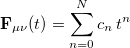
The Fock matrix elements $\ensuremath{\mathbf{F}}_{\mu \nu }$ in the atomic orbital basis are oscillatory functions of the time $t$ , and Q-Chem’s extrapolation procedure fits these oscillations to a power series in $t$ :

$\begin{equation} {\rm {\bf F}}_{\mu \nu } (t)=\sum \limits _{n=0}^ N {c_ n \, } t^ n \end{equation}$

(9.9)

The $N+1$ extrapolation coefficients $c_ n$ are determined by a fit to a set of $M$ Fock matrices retained from previous time steps. Fock matrix extrapolation can significantly reduce the number of SCF iterations required at each time step, but for low-order extrapolations, or if SCF_CONVERGENCE is set too small, a systematic drift in the total energy may be observed. Benchmark calculations testing the limits of energy conservation can be found in Ref. Herbert:2005, and demonstrate that numerically exact classical dynamics (without energy drift) can be obtained at significantly reduced cost.

Fock matrix extrapolation is requested by specifying values for $N$ and $M$ , as in the form of the following two $rem variables:

FOCK_EXTRAP_ORDER

Specifies the polynomial order $N$ for Fock matrix extrapolation.

TYPE:

INTEGER

DEFAULT:

0

Do not perform Fock matrix extrapolation.

OPTIONS:

$N$

Extrapolate using an $N$ th-order polynomial ( $N > 0$ ).

RECOMMENDATION:

None

FOCK_EXTRAP_POINTS

Specifies the number $M$ of old Fock matrices that are retained for use in extrapolation.

TYPE:

INTEGER

DEFAULT:

0

Do not perform Fock matrix extrapolation.

OPTIONS:

$M$

Save $M$ Fock matrices for use in extrapolation $(M > N)$

RECOMMENDATION:

Higher-order extrapolations with more saved Fock matrices are faster and conserve energy better than low-order extrapolations, up to a point. In many cases, the scheme ( $N$ = 6, $M$ = 12), in conjunction with SCF_CONVERGENCE = 6, is found to provide about a 50% savings in computational cost while still conserving energy.

When nuclear forces are computed using underlying electronic structure methods with non-optimized orbitals (such as MP2), a set of response equations must be solved [441]. While these equations are linear, their dimensionality necessitates an iterative solution [442, 443], which, in practice, looks much like the SCF equations. Extrapolation is again useful here [207], and the syntax for $Z$ -vector (response) extrapolation is similar to Fock extrapolation:

Z_EXTRAP_ORDER

Specifies the polynomial order $N$ for Z-vector extrapolation.

TYPE:

INTEGER

DEFAULT:

0

Do not perform $Z$ -vector extrapolation.

OPTIONS:

$N$

Extrapolate using an $N$ th-order polynomial ( $N > 0$ ).

RECOMMENDATION:

None

Z_EXTRAP_POINTS

Specifies the number $M$ of old $Z$ -vectors that are retained for use in extrapolation.

TYPE:

INTEGER

DEFAULT:

0

Do not perform response equation extrapolation.

OPTIONS:

$M$

Save $M$ previous $Z$ -vectors for use in extrapolation $(M>N)$

RECOMMENDATION:

Using the default $Z$ -vector convergence settings, a (4,2)=( $M$ , $N$ ) extrapolation was shown to provide the greatest speedup. At this setting, a 2–3-fold reduction in iterations was demonstrated.

Assuming decent conservation, a BOMD calculation represents exact classical dynamics on the Born-Oppenheimer potential energy surface. In contrast, so-called extended Lagrangian molecular dynamics (ELMD) methods make an approximation to exact classical dynamics in order to expedite the calculations. ELMD methods—of which the most famous is Car–Parrinello molecular dynamics—introduce a fictitious dynamics for the electronic (orbital) degrees of freedom, which are then propagated alongside the nuclear degrees of freedom, rather than optimized at each time step as they are in a BOMD calculation. The fictitious electronic dynamics is controlled by a fictitious mass parameter $\mu$ , and the value of $\mu$ controls both the accuracy and the efficiency of the method. In the limit of small $\mu$ the nuclei and the orbitals propagate adiabatically, and ELMD mimics true classical dynamics. Larger values of $\mu$ slow down the electronic dynamics, allowing for larger time steps (and more computationally efficient dynamics), at the expense of an ever-greater approximation to true classical dynamics.

Q-Chem’s ELMD algorithm is based upon propagating the density matrix, expressed in a basis of atom-centered Gaussian orbitals, along shortest-distance paths (geodesics) of the manifold of allowed density matrices $\ensuremath{\mathbf{P}}$ . Idempotency of $\ensuremath{\mathbf{P}}$ is maintained at every time step, by construction, and thus our algorithm requires neither density matrix purification, nor iterative solution for Lagrange multipliers (to enforce orthogonality of the molecular orbitals). We call this procedure “curvy steps” ELMD [206], and in a sense it is a time-dependent implementation of the GDM algorithm (Section 4.5) for converging SCF single-point calculations.

The extent to which ELMD constitutes a significant approximation to BOMD continues to be debated. When assessing the accuracy of ELMD, the primary consideration is whether there exists a separation of time scales between nuclear oscillations, whose time scale $\tau _{\ensuremath{\mathrm{nuc}}}$ is set by the period of the fastest vibrational frequency, and electronic oscillations, whose time scale $\tau _{\ensuremath{\mathrm{elec}}}$ may be estimated according to [206]

$\begin{equation} \tau _{\ensuremath{\mathrm{elec}}} \geq \sqrt {\mu /(\varepsilon _{\ensuremath{\mathrm{LUMO}}} -\varepsilon _{\ensuremath{\mathrm{HOMO}}} )} \quad \end{equation}$

(9.10)

A conservative estimate, suggested in Ref. Herbert:2004, is that essentially exact classical dynamics is attained when $\tau _{\ensuremath{\mathrm{nuc}} }>$ 10 $\tau _{\ensuremath{\mathrm{elec}}}$ . In practice, we recommend careful benchmarking to insure that ELMD faithfully reproduces the BOMD observables of interest.

Due to the existence of a fast time scale $\tau _{\ensuremath{\mathrm{elec}}}$ , ELMD requires smaller time steps than BOMD. When BOMD is combined with Fock matrix extrapolation to accelerate convergence, it is no longer clear that ELMD methods are substantially more efficient, at least in Gaussian basis sets [439, 440].

The following $rem variables are required for ELMD jobs:

AIMD_FICT_MASS

Specifies the value of the fictitious electronic mass $\mu$ , in atomic units, where $\mu$ has dimensions of (energy) $\times$ (time) $^{2}$ .

TYPE:

INTEGER

DEFAULT:

None

OPTIONS:

User-specified

RECOMMENDATION:

Values in the range of 50–200 a.u. have been employed in test calculations; consult [206] for examples and discussion.

Additional job control variables for ab initio molecular dynamics.

AIMD_INIT_VELOC

Specifies the method for selecting initial nuclear velocities.

TYPE:

STRING

DEFAULT:

None

OPTIONS:

THERMAL

Random sampling of nuclear velocities from a Maxwell-Boltzmann

distribution. The user must specify the temperature in Kelvin via

the $rem variable AIMD_TEMP.

ZPE

Choose velocities in order to put zero-point vibrational energy into

each normal mode, with random signs. This option requires that a

frequency job to be run beforehand.

QUASICLASSICAL

Puts vibrational energy into each normal mode. In contrast to the

ZPE option, here the vibrational energies are sampled from a

Boltzmann distribution at the desired simulation temperature. This

also triggers several other options, as described below.

RECOMMENDATION:

This variable need only be specified in the event that velocities are not specified explicitly in a $velocity section.

AIMD_MOMENTS

Requests that multipole moments be output at each time step.

TYPE:

INTEGER

DEFAULT:

0

Do not output multipole moments.

OPTIONS:

$n$

Output the first $n$ multipole moments.

RECOMMENDATION:

None

AIMD_TEMP

Specifies a temperature (in Kelvin) for Maxwell-Boltzmann velocity sampling.

TYPE:

INTEGER

DEFAULT:

None

OPTIONS:

User-specified number of Kelvin.

RECOMMENDATION:

This variable is only useful in conjunction with AIMD_INIT_VELOC = THERMAL. Note that the simulations are run at constant energy, rather than constant temperature, so the mean nuclear kinetic energy will fluctuate in the course of the simulation.

DEUTERATE

Requests that all hydrogen atoms be replaces with deuterium.

TYPE:

LOGICAL

DEFAULT:

FALSE

Do not replace hydrogens.

OPTIONS:

TRUE

Replace hydrogens with deuterium.

RECOMMENDATION:

Replacing hydrogen atoms reduces the fastest vibrational frequencies by a factor of 1.4, which allow for a larger fictitious mass and time step in ELMD calculations. There is no reason to replace hydrogens in BOMD calculations.

9.9.1 Examples

Example 9.200 Simulating thermal fluctuations of the water dimer at 298 K.

$molecule
   0  1
   O   1.386977   0.011218   0.109098
   H   1.748442   0.720970  -0.431026
   H   1.741280  -0.793653  -0.281811
   O  -1.511955  -0.009629  -0.120521
   H  -0.558095   0.008225   0.047352
   H  -1.910308   0.077777   0.749067
$end

$rem
   JOBTYPE              aimd
   AIMD_METHOD          bomd
   METHOD               b3lyp
   BASIS                6-31g*
   TIME_STEP            20        (20 a.u. = 0.48 fs) 
   AIMD_STEPS           1000
   AIMD_INIT_VELOC      thermal
   AIMD_TEMP            298
   FOCK_EXTRAP_ORDER    6         request Fock matrix extrapolation
   FOCK_EXTRAP_POINTS   12 
$end

Example 9.201 Propagating $\rm F-(H_2O)_4$ on its first excited-state potential energy surface, calculated at the CIS level.

$molecule
   -1   1
   O  -1.969902  -1.946636   0.714962
   H  -2.155172  -1.153127   1.216596
   H  -1.018352  -1.980061   0.682456
   O  -1.974264   0.720358   1.942703
   H  -2.153919   1.222737   1.148346
   H  -1.023012   0.684200   1.980531
   O  -1.962151   1.947857  -0.723321
   H  -2.143937   1.154349  -1.226245
   H  -1.010860   1.980414  -0.682958
   O  -1.957618  -0.718815  -1.950659
   H  -2.145835  -1.221322  -1.158379
   H  -1.005985  -0.682951  -1.978284
   F   1.431477   0.000499   0.010220
$end

$rem
   JOBTYPE           aimd
   AIMD_METHOD       bomd
   METHOD            hf
   BASIS             6-31+G*
   ECP               SRLC
   PURECART          1111
   CIS_N_ROOTS       3
   CIS_TRIPLETS      false
   CIS_STATE_DERIV   1         propagate on first excited state
   AIMD_INIT_VELOC   thermal
   AIMD_TEMP         150
   TIME_STEP         25
   AIMD_STEPS        827      (500 fs)
$end

Example 9.202 Simulating vibrations of the NaCl molecule using ELMD.

$molecule
   0  1
   Na   0.000000   0.000000  -1.742298 
   Cl   0.000000   0.000000   0.761479
$end

$rem
   JOBTYPE    freq
   METHOD     b3lyp
   ECP        sbkjc
$end

@@@

$molecule
   read
$end

$rem
   JOBTYPE           aimd
   METHOD            b3lyp
   ECP               sbkjc
   TIME_STEP         14
   AIMD_STEPS        500
   AIMD_METHOD       curvy
   AIMD_FICT_MASS    360
   AIMD_INIT_VELOC   zpe
$end

9.9.2 AIMD with Correlated Wavefunctions

While the number of time steps required in most AIMD trajectories dictates that economical (typically SCF-based) underlying electronic structure methods are required, other methods are also now possible. Any method with available analytic forces can be utilized for BOMD. Currently, Q-Chem can perform AIMD simulations with HF, DFT, MP2, RI-MP2, CCSD, and CCSD(T). The RI-MP2 method, especially when combined with Fock matrix and response equation extrapolation, is particularly effective as an alternative to DFT-based dynamics.

9.9.3 Vibrational Spectra

The inherent nuclear motion of molecules is experimentally observed by the molecules’ response to impinging radiation. This response is typically calculated within the mechanical and electrical harmonic approximations (second derivative calculations) at critical-point structures. Spectra, including anharmonic effects, can also be obtained from dynamics simulations. These spectra are generated from dynamical response functions, which involve the Fourier transform of autocorrelation functions. Q-Chem can provide both the vibrational spectral density from the velocity autocorrelation function

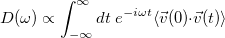$\begin{equation} D(\omega ) \propto \int _{-\infty }^{\infty } dt\ e^{-i\omega t} \langle \vec{v}(0){\cdot }\vec{v}(t)\rangle \end{equation}$

(9.11)

and infrared absorption intensity from the dipole autocorrelation function

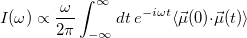$\begin{equation} I(\omega ) \propto \frac{\omega }{2\pi }\int _{-\infty }^{\infty } dt\ e^{-i\omega t} \langle \vec{\mu }(0){\cdot }\vec{\mu }(t)\rangle \end{equation}$

(9.12)

These two features are activated by the AIMD_NUCL_VACF_POINTS and AIMD_NUCL_DACF_POINTS keywords, respectively, where values indicate the number of data points to include in the correlation function. Furthermore, the AIMD_NUCL_SAMPLE_RATE keyword controls the frequency at which these properties are sampled (entered as number of time steps). These spectra—generated at constant energy—should be averaged over a suitable distribution of initial conditions. The averaging indicated in the expressions above, for example, should be performed over a Boltzmann distribution of initial conditions.

Note that dipole autocorrelation functions can exhibit contaminating information if the molecule is allowed to rotate/translate. While the initial conditions in Q-Chem remove translation and rotation, numerical noise in the forces and propagation can lead to translation and rotation over time. The trans/rot correction in Q-Chem is activated by the PROJ_TRANSROT keyword.

AIMD_NUCL_VACF_POINTS

Number of time points to utilize in the velocity autocorrelation function for an AIMD trajectory

TYPE:

INTEGER

DEFAULT:

0

OPTIONS:

0

Do not compute velocity autocorrelation function.

$1\leq n \leq \mbox{{\small AIMD\_ STEPS}}$

Compute velocity autocorrelation function for last $n$

time steps of the trajectory.

RECOMMENDATION:

If the VACF is desired, set equal to AIMD_STEPS.

AIMD_NUCL_DACF_POINTS

Number of time points to utilize in the dipole autocorrelation function for an AIMD trajectory

TYPE:

INTEGER

DEFAULT:

0

OPTIONS:

0

Do not compute dipole autocorrelation function.

$1\leq n \leq \mbox{{\small AIMD\_ STEPS}}$

Compute dipole autocorrelation function for last $n$

timesteps of the trajectory.

RECOMMENDATION:

If the DACF is desired, set equal to AIMD_STEPS.

AIMD_NUCL_SAMPLE_RATE

The rate at which sampling is performed for the velocity and/or dipole autocorrelation function(s). Specified as a multiple of steps; i.e., sampling every step is 1.

TYPE:

INTEGER

DEFAULT:

None.

OPTIONS:

$1\leq n \leq \mbox{{\small AIMD\_ STEPS}}$

Update the velocity/dipole autocorrelation function

every $n$ steps.

RECOMMENDATION:

Since the velocity and dipole moment are routinely calculated for ab initio methods, this variable should almost always be set to 1 when the VACF/DACF are desired.

PROJ_TRANSROT

Removes translational and rotational drift during AIMD trajectories.

TYPE:

LOGICAL

DEFAULT:

FALSE

OPTIONS:

FALSE

Do not apply translation/rotation corrections.

TRUE

Apply translation/rotation corrections.

RECOMMENDATION:

When computing spectra (see AIMD_NUCL_DACF_POINTS, for example), this option can be utilized to remove artificial, contaminating peaks stemming from translational and/or rotational motion. Recommend setting to TRUE for all dynamics-based spectral simulations.

9.9.4 Quasi-Classical Molecular Dynamics

Molecular dynamics simulations based on quasi classical trajectories (QCT-MD) [444, 445, 446] put vibrational energy into each mode in the initial velocity setup step. We (as well as others [447]) have found that this can improve on the results of purely classical simulations, for example in the calculation of photoelectron [448] or infrared spectra [449]. Improvements include better agreement of spectral linewidths with experiment at lower temperatures or better agreement of vibrational frequencies with anharmonic calculations.

The improvements at low temperatures can be understood by recalling that even at low temperature there is nuclear motion due to zero-point motion. This is included in the quasi-classical initial velocities, thus leading to finite peak widths even at low temperatures. In contrast to that the classical simulations yield zero peak width in the low temperature limit, because the thermal kinetic energy goes to zero as temperature decreases. Likewise, even at room temperature the quantum vibrational energy for high-frequency modes is often significantly larger than the classical kinetic energy. QCT-MD therefore typically samples regions of the potential energy surface that are higher in energy and thus more anharmonic than the low-energy regions accessible to classical simulations. These two effects can lead to improved peak widths as well as a more realistic sampling of the anharmonic parts of the potential energy surface. However, the QCT-MD method also has important limitations which are described below and that the user has to monitor for carefully.

In our QCT-MD implementation the initial vibrational quantum numbers are generated as random numbers sampled from a vibrational Boltzmann distribution at the desired simulation temperature. In order to enable reproducibility of the results, each trajectory (and thus its set of vibrational quantum numbers) is denoted by a unique number using the AIMD_QCT_WHICH_TRAJECTORY variable. In order to loop over different initial conditions, run trajectories with different choices for AIMD_QCT_WHICH_TRAJECTORY. It is also possible to assign initial velocities corresponding to an average over a certain number of trajectories by choosing a negative value. Further technical details of our QCT-MD implementation are described in detail in Appendix A of Ref. Lambrecht:2011.

AIMD_QCT_WHICH_TRAJECTORY

Picks a set of vibrational quantum numbers from a random distribution.

TYPE:

INTEGER

DEFAULT:

1

OPTIONS:

$n$

Picks the $n$ th set of random initial velocities.

$-n$

Uses an average over $n$ random initial velocities.

RECOMMENDATION:

Pick a positive number if you want the initial velocities to correspond to a particular set of vibrational occupation numbers and choose a different number for each of your trajectories. If initial velocities are desired that corresponds to an average over $n$ trajectories, pick a negative number.

Below is a simple example input for running a QCT-MD simulation of the vibrational spectrum of water. Most input variables are the same as for classical MD as described above. The use of quasi-classical initial conditions is triggered by setting the AIMD_INIT_VELOC variable to QUASICLASSICAL.

Example 9.203 Simulating the IR spectrum of water using QCT-MD.

$comment
  Don't forget to run a frequency calculation prior to this job.
$end

$molecule
  0  1
  O           0.000000    0.000000    0.520401
  H          -1.475015    0.000000   -0.557186
  H           1.475015    0.000000   -0.557186
$end


$rem
  jobtype     aimd
  input_bohr  true
  method      hf
  basis       3-21g
  scf_convergence 6
  ! AIMD input
  time_step                      20      (in atomic units)
  aimd_steps                  12500      6 ps total simulation time
  aimd_temp                      12
  aimd_print                      2
  fock_extrap_order               6      Use a 6th-order extrapolation
  fock_extrap_points             12      of the previous 12 Fock matrices
  ! IR spectral sampling
  aimd_moments                    1
  aimd_nucl_sample_rate           5
  aimd_nucl_vacf_points        1000
  ! QCT-specific settings
  aimd_init_veloc    quasiclassical
  aimd_qct_which_trajectory       1      Loop over several values to get
                                         the correct Boltzmann distribution.
$end

Other types of spectra can be calculated by calculating spectral properties along the trajectories. For example, we observed that photoelectron spectra can be approximated quite well by calculating vertical detachment energies (VDEs) along the trajectories and generating the spectrum as a histogram of the VDEs [448]. We have included several simple scripts in the $QC/aimdman/tools subdirectory that we hope the user will find helpful and that may serve as the basis for developing more sophisticated tools. For example, we include scripts that allow to perform calculations along a trajectory (md_calculate_along_trajectory) or to calculate vertical detachment energies along a trajectory (calculate_rel_energies).

Another application of the QCT code is to generate random geometries sampled from the vibrational wavefunction via a Monte Carlo algorithm. This is triggered by setting both the AIMD_QCT_INITPOS and AIMD_QCT_WHICH_TRAJECTORY variables to negative numbers, say $-m$ and $-n$ , and setting AIMD_STEPS to zero. This will generate $m$ random geometries sampled from the vibrational wavefunction corresponding to an average over $n$ trajectories at the user-specified simulation temperature.

AIMD_QCT_INITPOS

Chooses the initial geometry in a QCT-MD simulation.

TYPE:

INTEGER

DEFAULT:

0

OPTIONS:

$0$

Use the equilibrium geometry.

$n$

Picks a random geometry according to the harmonic vibrational wavefunction.

$-n$

Generates $n$ random geometries sampled from

the harmonic vibrational wavefunction.

RECOMMENDATION:

None.

For systems that are described well within the harmonic oscillator model and for properties that rely mainly on the ground-state dynamics, this simple MC approach may yield qualitatively correct spectra. In fact, one may argue that it is preferable over QCT-MD for describing vibrational effects at very low temperatures, since the geometries are sampled from a true quantum distribution (as opposed to classical and quasiclassical MD). We have included another script in the aimdman/tools directory to help with the calculation of vibrationally averaged properties (monte_geom).

Example 9.204 MC sampling of the vibrational wavefunction for HCl.

$comment
  Generates 1000 random geometries for HCl based on the harmonic vibrational 
  wavefunction at 1 Kelvin. The wavefunction is averaged over 1000
  sets of random vibrational quantum numbers (\ie{}, the ground state in
  this case due to the low temperature).
$end

$molecule
  0 1
  H           0.000000    0.000000   -1.216166
  Cl          0.000000    0.000000    0.071539
$end

$rem
  jobtype                              aimd
  method                              B3LYP
  basis                          6-311++G**
  scf_convergence                         1
  SKIP_SCFMAN                             1
  maxscf                                  0
  xc_grid                                 1
  time_step                              20     (in atomic units)
  aimd_steps                              0
  aimd_init_veloc            quasiclassical
  aimd_qct_vibseed                        1
  aimd_qct_velseed                        2
  aimd_temp                               1     (in Kelvin)
  ! set aimd_qct_which_trajectory to the desired
  ! trajectory number
  aimd_qct_which_trajectory           -1000
  aimd_qct_initpos                    -1000
$end

It is also possible make some modes inactive, i.e., to put vibrational energy into a subset of modes (all other are set to zero). The list of active modes can be specified using the $qct_active_modes section. Furthermore, the vibrational quantum numbers for each mode can be specified explicitly using the $qct_vib_distribution keyword. It is also possible to set the phases using $qct_vib_phase (allowed values are 1 and -1). Below is a simple sample input:

Example 9.205 User control over the QCT variables.

$comment
  Makes the 1st vibrational mode QCT-active; all other ones receive zero
  kinetic energy. We choose the vibrational ground state and a positive
  phase for the velocity. 
$end

...

$qct_active_modes
  1
$end

$qct_vib_distribution
  0
$end

$qct_vib_phase
  1
$end

...

Finally we turn to a brief description of the limitations of QCT-MD. Perhaps the most severe limitation stems from the so-called “kinetic energy spilling problem” (see, e.g., Ref. Czako:2010), which means that there can be an artificial transfer of kinetic energy between modes. This can happen because the initial velocities are chosen according to quantum energy levels, which are usually much higher than those of the corresponding classical systems. Furthermore, the classical equations of motion also allow for the transfer of non-integer multiples of the zero-point energy between the modes, which leads to different selection rules for the transfer of kinetic energy. Typically, energy spills from high-energy into low-energy modes, leading to spurious ”hot” dynamics. A second problem is that QCT-MD is actually based on classical Newtonian dynamics, which means that the probability distribution at low temperatures can be qualitatively wrong compared to the true quantum distribution [448].

We have implemented a routine that monitors the kinetic energy within each normal mode along the trajectory and that is automatically switched on for quasiclassical simulations. It is thus possible to monitor for trajectories in which the kinetic energy in one or more modes becomes significantly larger than the initial energy. Such trajectories should be discarded (see Ref. Czako:2010 for a different approach to the zero-point leakage problem). Furthermore, this monitoring routine prints the squares of the (harmonic) vibrational wavefunction along the trajectory. This makes it possible to weight low-temperature results with the harmonic quantum distribution to alleviate the failure of classical dynamics for low temperatures.

BOMD	Born-Oppenheimer molecular dynamics.
CURVY	Curvy-steps Extended Lagrangian molecular dynamics.

THERMAL	Random sampling of nuclear velocities from a Maxwell-Boltzmann
	distribution. The user must specify the temperature in Kelvin via
	the $rem variable AIMD_TEMP.
ZPE	Choose velocities in order to put zero-point vibrational energy into
	each normal mode, with random signs. This option requires that a
	frequency job to be run beforehand.
QUASICLASSICAL	Puts vibrational energy into each normal mode. In contrast to the
	ZPE option, here the vibrational energies are sampled from a
	Boltzmann distribution at the desired simulation temperature. This
	also triggers several other options, as described below.

0	Do not compute velocity autocorrelation function.
$1\leq n \leq \mbox{{\small AIMD\_ STEPS}}$	Compute velocity autocorrelation function for last $n$
	time steps of the trajectory.

0	Do not compute dipole autocorrelation function.
$1\leq n \leq \mbox{{\small AIMD\_ STEPS}}$	Compute dipole autocorrelation function for last $n$
	timesteps of the trajectory.

$1\leq n \leq \mbox{{\small AIMD\_ STEPS}}$	Update the velocity/dipole autocorrelation function
	every $n$ steps.

FALSE	Do not apply translation/rotation corrections.
TRUE	Apply translation/rotation corrections.