9.10 Ab initio Path Integrals
Even in cases where the Born-Oppenheimer separation is valid, solving the electronic Schroedinger equation—Q-Chem’s main purpose—is still only half the battle. The remainder involves the solution of the nuclear Schroedinger equation for its resulting eigenvalues/functions. This half is typically treated by the harmonic approximation at critical points, but anharmonicity, tunneling, and low-frequency “floppy” motion can lead to extremely delocalized nuclear distributions, particularly for protons and non-covalently bonded systems.
While the Born-Oppenheimer separation allows for a local solution of the electronic problem (in nuclear space), the nuclear half of the Schroedinger equation is entirely non-local and requires the computation of potential energy surfaces over large regions of configuration space. Grid-based methods, therefore, scale exponentially with the number of degrees of freedom, and are quickly rendered useless for all but very small molecules.
For thermal, equilibrium distributions, the path integral (PI) formalism of Feynman provides both an elegant and computationally feasible alternative. The equilibrium partition function, for example, may be written as a trace of the thermal, configuration-space density matrix:
 |
 |
![$\displaystyle Tr\left[e^{-\beta \hat{H}}\right] $](images/img-1060.png) |
|||
 |
|
 |
(9.13) | ||
|
|
 |
Solving for the partition function directly in this form is equally difficult, as it still requires the eigenvalues/eigenstates of  . By inserting
  resolutions of the identity, however, this integral may be converted to the following form
 |
(9.14) |
While this additional integration appears to be a detriment, the ability to use a high-temperature ( ) form of the density matrix
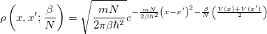 |
(9.15) |
renders this path-integral formulation a net win. By combining the  time slices, the partition function takes the following form (in 1-D):
|
|
![$\displaystyle \left(\frac{mN}{2\pi \beta \hbar ^2}\right)^{\frac{N}{2}} \int dx_1 \int dx_2 \cdots \int dx_ N e^{-\frac{\beta }{N} \left[ \frac{mN^2}{2\beta ^2\hbar ^2}\sum _ i^ N \left(x_ i - x_{i+1}\right)^2 + \sum _ i^ N V(x_ i)\right]} $](images/img-1066.png) |
|||
|
 |
 |
(9.16) |
with the implied cyclic condition  . Here,
  is the potential function on which the “beads” move (the electronic potential generated by Q-Chem). The resulting integral, as shown in the last line above, is nothing more than a classical configuration integral in an -dimensional space. The effective potential appearing above describes an -bead “ring polymer,” of which neighboring beads are harmonically coupled. The exponentially scaling, non-local nuclear problem has, therefore, been mapped onto an entirely classical problem, which is amenable to standard treatments of configuration sampling. These methods typically involve (thermostated) molecular dynamics or Monte Carlo sampling; only the latter is currently implemented in Q-Chem. Importantly, is reasonably small when the temperature is not too low: room-temperature systems involving H atoms typically are converged with roughly 30 beads. Therefore, fully quantum mechanical nuclear distributions may be obtained at a cost only roughly 30 times a classical simulation.
Path integral Monte Carlo (PIMC) is an entirely new job type in Q-Chem and is activated by setting JOBTYP to PIMC.
9.10.1 Classical Sampling
The 1-bead limit of the above expressions is simply classical configuration sampling. When the temperature (controlled by the PIMC_TEMP keyword) is high or only heavy atoms are involved, the classical limit is often appropriate. The path integral machinery (with 1 “bead”) may be utilized to perform classical Boltzmann sampling. The 1D partition function, for example, is simply
 |
(9.17) |
9.10.2 Quantum Sampling
Using more beads includes more quantum mechanical delocalization (at a cost of roughly times the classical analog). This main input variable—the number of time slices (beads)—is controlled by the PIMC_NBEADSPERATOM keyword. The ratio of the inverse temperature to beads () dictates convergence with respect to the number of beads, so as the temperature is lowered, a concomitant increase in the number of beads is required.
Integration over configuration space is performed by Metropolis Monte Carlo (MC). The number of MC steps is controlled by the PIMC_MCMAX keyword and should typically be at least  , depending on the desired level of statistical convergence. A warmup run, in which the ring polymer is allowed to equilibrate (without accumulating statistics) can be performed by setting the PIMC_WARMUP_MCMAX keyword.
Much like ab initio molecular dynamics simulations, the main results of PIMC jobs in Q-Chem are not in the job output file. Rather, they are compiled in the “PIMC” subdirectory of the user’s scratch directory ($QCSCRATCH/PIMC). Therefore, PIMC jobs should always be run with the -save option. The output files do contain some useful information, however, including a basic data analysis of the simulation. Average energies (thermodynamic estimator), bond lengths (less than 5), bond length standard deviations and errors are printed at the end of the output file. The $QCSCRATCH/PIMC directory additionally contains the following files:
BondAves: running average of bond lengths for convergence testing.
BondBins: normalized distribution of significant bond lengths, binned within 5 standard deviations of the average bond length.
ChainCarts: human-readable file of configuration coordinates, likely to be used for further, external statistical analysis. This file can get quite large, so be sure to provide enough scratch space!
ChainView.xyz: xyz-formatted file for viewing the ring-polymer sampling in an external visualization program. (The sampling is performed such that the center of mass of the ring polymer system remains centered.)
Vcorr: potential correlation function for the assessment of statistical correlations in the sampling.
In each of the above files, the first few lines contain a description of the ordering of the data.
One of the unfortunate rites of passage in PIMC usage is the realization of the ramifications of the stiff bead-bead interactions as convergence (with respect to ) is approached. Nearing convergence—where quantum mechanical results are correct—the length of statistical correlations grows enormously, and special sampling techniques are required to avoid long (or non-convergent) simulations. Cartesian displacements or normal-mode displacements of the ring polymer lead to this severe stiffening. While both of these naive sampling schemes are available in Q-Chem, they are not recommended. Rather, the free-particle (harmonic bead-coupling) terms in the path integral action can be sampled directly. Several schemes are available for this purpose. Q-Chem currently utilizes the simplest of these options: Levy flights. An  -bead snippet (
 ) of the ring polymer is first chosen at random, with the length controlled by the PIMC_SNIP_LENGTH keyword. Between the endpoints of this snippet, a free-particle path is generated by a Levy construction, which exactly samples the free-particle part of the action. Subsequent Metropolis testing of the resulting potential term—for which only the potential on the moved beads is required—then dictates acceptance.
Two measures of the sampling efficiency are provided in the job output file. The lifetime of the potential autocorrelation function  is provided in terms of the number of MC steps,
  . This number indicates the number of configurations that are statically correlated. Similarly, the mean-square displacement between MC configurations is also provided. Maximizing this number and/or minimizing the statistical lifetime leads to efficient sampling. Note that the optimally efficient acceptance rate may not be 50% in MC simulations. In Levy flights, the only variable controlling acceptance and sampling efficiency is the length of the snippet. The statistical efficiency can be obtained from relatively short runs, during which the length of the Levy snippet should be optimized by the user.
PIMC_NBEADSPERATOM
Number of path integral time slices (“beads”) used on each atom of a PIMC simulation.
TYPE:
INTEGER
DEFAULT:
None.
OPTIONS:
1
Perform classical Boltzmann sampling.
1
Perform quantum-mechanical path integral sampling.
RECOMMENDATION:
This variable controls the inherent convergence of the path integral simulation. The 1-bead limit is purely classical sampling; the infinite-bead limit is exact quantum mechanical sampling. Using 32 beads is reasonably converged for room-temperature simulations of molecular systems.
PIMC_TEMP
Temperature, in Kelvin (K), of path integral simulations.
TYPE:
INTEGER
DEFAULT:
None.
OPTIONS:
User-specified number of Kelvin for PIMC or classical MC simulations.
RECOMMENDATION:
None.
PIMC_MCMAX
Number of Monte Carlo steps to sample.
TYPE:
INTEGER
DEFAULT:
None.
OPTIONS:
User-specified number of steps to sample.
RECOMMENDATION:
This variable dictates the statistical convergence of MC/PIMC simulations. Recommend setting to at least 100000 for converged simulations.
PIMC_WARMUP_MCMAX
Number of Monte Carlo steps to sample during an equilibration period of MC/PIMC simulations.
TYPE:
INTEGER
DEFAULT:
None.
OPTIONS:
User-specified number of steps to sample.
RECOMMENDATION:
Use this variable to equilibrate the molecule/ring polymer before collecting production statistics. Usually a short run of roughly 10% of PIMC_MCMAX is sufficient.
PIMC_MOVETYPE
Selects the type of displacements used in MC/PIMC simulations.
TYPE:
INTEGER
DEFAULT:
0
OPTIONS:
0
Cartesian displacements of all beads, with occasional (1%) center-of-mass moves.
1
Normal-mode displacements of all modes, with occasional (1%) center-of-mass moves.
2
Levy flights without center-of-mass moves.
RECOMMENDATION:
Except for classical sampling (MC) or small bead-number quantum sampling (PIMC), Levy flights should be utilized. For Cartesian and normal-mode moves, the maximum displacement is adjusted during the warmup run to the desired acceptance rate (controlled by PIMC_ACCEPT_RATE). For Levy flights, the acceptance is solely controlled by PIMC_SNIP_LENGTH.
PIMC_ACCEPT_RATE
Acceptance rate for MC/PIMC simulations when Cartesian or normal-mode displacements are utilized.
TYPE:
INTEGER
DEFAULT:
None
OPTIONS:

User-specified rate, given as a whole-number percentage.
RECOMMENDATION:
Choose acceptance rate to maximize sampling efficiency, which is typically signified by the mean-square displacement (printed in the job output). Note that the maximum displacement is adjusted during the warmup run to achieve roughly this acceptance rate.
PIMC_SNIP_LENGTH
Number of “beads” to use in the Levy flight movement of the ring polymer.
TYPE:
INTEGER
DEFAULT:
None
OPTIONS:

User-specified length of snippet.
RECOMMENDATION:
Choose the snip length to maximize sampling efficiency. The efficiency can be estimated by the mean-square displacement between configurations, printed at the end of the output file. This efficiency will typically, however, be a trade-off between the mean-square displacement (length of statistical correlations) and the number of beads moved. Only the moved beads require recomputing the potential, i.e., a call to Q-Chem for the electronic energy. (Note that the endpoints of the snippet remain fixed during a single move, so
beads are actually moved for a snip length of
9.10.3 Examples
Example 9.206 Path integral Monte Carlo simulation of H at room temperature
$molecule
   0  1
   H
   H 1 0.75
$end

$rem
   JOBTYPE              pimc
   METHOD               hf
   BASIS                sto-3g
   PIMC_TEMP            298
   PIMC_NBEADSPERATOM   32
   PIMC_WARMUP_MCMAX    10000     !Equilibration run
   PIMC_MCMAX           100000    !Production run
   PIMC_MOVETYPE        2         !Levy flights
   PIMC_SNIP_LENGTH     10        !Moves 8 beads per MC step (10-endpts)
$end
Example 9.207 Classical Monte Carlo simulation of a water molecule at 500K
$molecule
   0  1
   H
   O 1 1.0
   H 2 1.0 1 104.5
$end

$rem
   JOBTYPE              pimc
   METHOD               rimp2
   BASIS                cc-pvdz
   AUX_BASIS            rimp2-cc-pvdz
   PIMC_TEMP            500
   PIMC_NBEADSPERATOM   1       !1 bead is classical sampling
   PIMC_WARMUP_MCMAX    10000   !Equilibration run
   PIMC_MCMAX           100000  !Production run
   PIMC_MOVETYPE        0       !Cartesian displacements (ok for 1 bead)
   PIMC_ACCEPT_RATE     40      !During warmup, adjusts step size to 40% acceptance
$end