4.12 Unconventional SCF Calculations
4.12.1 Polarized Atomic Orbital (PAO) Calculations
Polarized atomic orbital (PAO) calculations are an interesting unconventional SCF method, in which the molecular orbitals and the density matrix are not expanded directly in terms of the basis of atomic orbitals. Instead, an intermediate molecule-optimized minimal basis of polarized atomic orbitals (PAOs) is used [306]. The polarized atomic orbitals are defined by an atom-blocked linear transformation from the fixed atomic orbital basis, where the coefficients of the transformation are optimized to minimize the energy, at the same time as the density matrix is obtained in the PAO representation. Thus a PAO-SCF calculation is a constrained variational method, whose energy is above that of a full SCF calculation in the same basis. However, a molecule optimized minimal basis is a very compact and useful representation for purposes of chemical analysis, and it also has potential computational advantages in the context of MP2 or local MP2 calculations, as can be done after a PAO-HF calculation is complete to obtain the PAO-MP2 energy.
PAO-SCF calculations tend to systematically underestimate binding energies (since by definition the exact result is obtained for atoms, but not for molecules). In tests on the G2 database, PAO-B3LYP/6-311+G(2df,p) atomization energies deviated from full B3LYP/6-311+G(2df,p) atomization energies by roughly 20 kcal/mol, with the error being essentially extensive with the number of bonds. This deviation can be reduced to only 0.5 kcal/mol with the use of a simple non-iterative second order correction for “beyond-minimal basis” effects [307]. The second order correction is evaluated at the end of each PAO-SCF calculation, as it involves negligible computational cost. Analytical gradients are available using PAOs, to permit structure optimization. For additional discussion of the PAO-SCF method and its uses, see the references cited above.
Calculations with PAOs are determined controlled by the following $rem variables. PAO_METHOD = PAO invokes PAO-SCF calculations, while the algorithm used to iterate the PAOs can be controlled with PAO_ALGORITHM.
PAO_ALGORITHM
Algorithm used to optimize polarized atomic orbitals (see PAO_METHOD)
TYPE:
INTEGER
DEFAULT:
0
OPTIONS:
0
Use efficient (and riskier) strategy to converge PAOs.
1
Use conservative (and slower) strategy to converge PAOs.
RECOMMENDATION:
None
PAO_METHOD
Controls evaluation of polarized atomic orbitals (PAOs).
TYPE:
STRING
DEFAULT:
EPAO
For local MP2 calculations Otherwise no default.
OPTIONS:
PAO
Perform PAO-SCF instead of conventional SCF.
EPAO
Obtain EPAOs after a conventional SCF.
RECOMMENDATION:
None
4.12.2 SCF Meta-Dynamics
As the SCF equations are non-linear in the electron density, there are in theory very many solutions (i.e., sets of orbitals where the energy is stationary with respect to changes in the orbital subset). Most often sought is the solution with globally minimal energy as this is a variational upper bound to the true eigenfunction in this basis. The SCF methods available in Q-Chem allow the user to converge upon an SCF solution, and (using STABILITY_ANALYSIS) ensure it is a minimum, but there is no known method of ensuring that the found solution is a global minimum; indeed in systems with many low-lying energy levels the solution converged upon may vary considerably with initial guess.
SCF meta-dynamics [308] is a technique which can be used to locate multiple SCF solutions, and thus gain some confidence that the calculation has converged upon the global minimum. It works by searching out a solution to the SCF equations. Once found, the solution is stored, and a biasing potential added so as to avoid re-converging to the same solution. More formally, the distance between two solutions,  and
and  , can be expressed as
 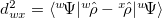 , where
  is a Slater determinant formed from the orthonormal orbitals,
  , of solution , and
  is the one-particle density operator for . This definition is equivalent to
  and is easily calculated.
 is bounded by 0 and the number of electrons, and can be taken as the distance between two solutions. As an example, any singly excited determinant from an SCF determinant (which will not in general be another SCF solution), would be a distance 1 away from it.
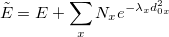
In a manner analogous to classical meta-dynamics, to bias against the set of previously located solutions, , we create a new Lagrangian,
 |
(4.114) |
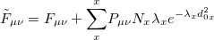
where  represents the present density. From this we may derive a new effective Fock matrix,
 |
(4.115) |
This may be used with very little modification within a standard DIIS procedure to locate multiple solutions. When close to a new solution, the biasing potential is removed so the location of that solution is not affected by it. If the calculation ends up re-converging to the same solution,  and
and  can be modified to avert this. Once a solution is found it is added to the list of solutions, and the orbitals mixed to provide a new guess for locating a different solution.
This process can be customized by the REM variables below. Both DIIS and GDM methods can be used, but it is advisable to turn on MOM when using DIIS to maintain the orbital ordering. Post-HF correlation methods can also be applied. By default they will operate for the last solution located, but this can be changed with the SCF_MINFIND_RUNCORR variable.
The solutions found through meta-dynamics also appear to be good approximations to diabatic surfaces where the electronic structure does not significantly change with geometry. In situations where there are such multiple electronic states close in energy, an adiabatic state may be produced by diagonalizing a matrix of these states - Configuration Interaction. As they are distinct solutions of the SCF equations, these states are non-orthogonal (one cannot be constructed as a single determinant made out of the orbitals of another), and so the CI is a little more complicated and is a non-orthogonal CI (NOCI). More information on NOCI can be found in Section 6.2.6.
SCF_SAVEMINIMA
Turn on SCF meta-dynamics and specify how many solutions to locate.
TYPE:
INTEGER
DEFAULT:
0
OPTIONS:
0
Do not use SCF meta-dynamics

Attempt to find
RECOMMENDATION:
Perform SCF Orbital meta-dynamics and attempt to locate
SCF_READMINIMA
Read in solutions from a previous SCF meta-dynamics calculation
TYPE:
INTEGER
DEFAULT:
0
OPTIONS:
Read in

Read in
RECOMMENDATION:
This may not actually locate all solutions required and will probably locate others too. The SCF will also stop when the number of solutions specified in SCF_SAVEMINIMA are found. Solutions from other geometries may also be read in and used as starting orbitals. If a solution is found and matches one that is read in within SCF_MINFIND_READDISTTHRESH, its orbitals are saved in that position for any future calculations. The algorithm works by restarting from the orbitals and density of a the minimum it is attempting to find. After 10 failed restarts (defined by SCF_MINFIND_RESTARTSTEPS), it moves to another previous minimum and attempts to locate that instead. If there are no minima to find, the restart does random mixing (with 10 times the normal random mixing parameter).
SCF_MINFIND_WELLTHRESH
Specify what SCF_MINFIND believes is the basin of a solution
TYPE:
INTEGER
DEFAULT:
5
OPTIONS:

RECOMMENDATION:
When the DIIS error is less than
SCF_MINFIND_RESTARTSTEPS
Restart with new orbitals if no minima have been found within this many steps
TYPE:
INTEGER
DEFAULT:
300
OPTIONS:
Restart after
RECOMMENDATION:
If the SCF calculation spends many steps not finding a solution, lowering this number may speed up solution-finding. If the system converges to solutions very slowly, then this number may need to be raised.
SCF_MINFIND_INCREASEFACTOR
Controls how the height of the penalty function changes when repeatedly trapped at the same solution
TYPE:
INTEGER
DEFAULT:
10100 meaning 1.01
OPTIONS:

corresponding to

RECOMMENDATION:
If the algorithm converges to a solution which corresponds to a previously located solution, increase both the normalization N and the width lambda of the penalty function there. Then do a restart.
SCF_MINFIND_INITLAMBDA
Control the initial width of the penalty function.
TYPE:
INTEGER
DEFAULT:
02000 meaning 2.000
OPTIONS:
corresponding to

RECOMMENDATION:
The initial inverse-width (i.e., the inverse-variance) of the Gaussian to place to fill solution’s well. Measured in electrons
. Increasing this will repeatedly converging on the same solution.
SCF_MINFIND_INITNORM
Control the initial height of the penalty function.
TYPE:
INTEGER
DEFAULT:
01000 meaning 1.000
OPTIONS:
RECOMMENDATION:
The initial normalization of the Gaussian to place to fill a well. Measured in hartrees.
SCF_MINFIND_RANDOMMIXING
Control how to choose new orbitals after locating a solution
TYPE:
INTEGER
DEFAULT:
00200 meaning .02 radians
OPTIONS:
RECOMMENDATION:
After locating an SCF solution, the orbitals are mixed randomly to move to a new position in orbital space. For each occupied and virtual orbital pair picked at random and rotate between them by a random angle between 0 and this. If this is negative then use exactly this number, e.g.,
will almost exactly swap orbitals. Any number
will cause the orbitals to be swapped exactly.
SCF_MINFIND_NRANDOMMIXES
Control how many random mixes to do to generate new orbitals
TYPE:
INTEGER
DEFAULT:
10
OPTIONS:
Perform
RECOMMENDATION:
This is the number of occupied/virtual pairs to attempt to mix, per separate density (i.e., for unrestricted calculations both alpha and beta space will get this many rotations). If this is negative then only mix the highest 25% occupied and lowest 25% virtuals.
SCF_MINFIND_READDISTTHRESH
The distance threshold at which to consider two solutions the same
TYPE:
INTEGER
DEFAULT:
00100 meaning 0.1
OPTIONS:
RECOMMENDATION:
The threshold to regard a minimum as the same as a read in minimum. Measured in electrons. If two minima are closer together than this, reduce the threshold to distinguish them.
SCF_MINFIND_MIXMETHOD
Specify how to select orbitals for random mixing
TYPE:
INTEGER
DEFAULT:
0
OPTIONS:
0
Random mixing: select from any orbital to any orbital.
1
Active mixing: select based on energy, decaying with distance from the Fermi level.
2
Active Alpha space mixing: select based on energy, decaying with distance from the
Fermi level only in the alpha space.
RECOMMENDATION:
Random mixing will often find very high energy solutions. If lower energy solutions are desired, use 1 or 2.
SCF_MINFIND_MIXENERGY
Specify the active energy range when doing Active mixing
TYPE:
INTEGER
DEFAULT:
00200 meaning 00.200
OPTIONS:
RECOMMENDATION:
The standard deviation of the Gaussian distribution used to select the orbitals for mixing (centered on the Fermi level). Measured in Hartree. To find less-excited solutions, decrease this value
SCF_MINFIND_RUNCORR
Run post-SCF correlated methods on multiple SCF solutions
TYPE:
INTEGER
DEFAULT:
0
OPTIONS:
If this is set
, then run correlation methods for all found SCF solutions.
RECOMMENDATION:
Post-HF correlation methods should function correctly with excited SCF solutions, but their convergence is often much more difficult owing to intruder states.