6.3 Time-Dependent Density Functional Theory (TDDFT)
6.3.1 Brief Introduction to TDDFT
Excited states may be obtained from density functional theory by time-dependent density functional theory [418, 419], which calculates poles in the response of the ground state density to a time-varying applied electric field. These poles are Bohr frequencies, or in other words the excitation energies. Operationally, this involves solution of an eigenvalue equation
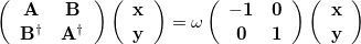 |
(6.15) |
where the elements of the matrix  similar to those used at the CIS level (Eq. eq:orbital-Hessian), but with an exchange-correlation correction [420]. Elements of
  are similar. Equation eq:TDDFT is solved iteratively for the lowest few excitation energies,
  . Alternatively, one can make a CIS-like Tamm-Dancoff approximation (TDA) [234], in which the “de-excitation” amplitudes
  are neglected, the matrix is not required, and Eq. eq:TDDFT reduces to
  .
.
TDDFT is popular because its computational cost is roughly similar to that of the simple CIS method, but a description of differential electron correlation effects is implicit in the method. It is advisable to only employ TDDFT for low-lying valence excited states that are below the first ionization potential of the molecule [418], or more conservatively, below the first Rydberg state, and in such cases the valence excitation energies are often remarkably improved relative to CIS, with an accuracy of  0.3 eV for many functionals [421]. The calculation of the nuclear gradients of full TDDFT and within the TDA is implemented [422].
On the other hand, standard density functionals do not yield a potential with the correct long-range Coulomb tail, owing to the so-called self-interaction problem, and therefore excitation energies corresponding to states that sample this tail (e.g., diffuse Rydberg states and some charge transfer excited states) are not given accurately [233, 423, 194]. The extent to which a particular excited state is characterized by charge transfer can be assessed using an a spatial overlap metric proposed by Peach, Benfield, Helgaker, and Tozer (PBHT) [424]. (However, see Ref. Richard:2011 for a cautionary note regarding this metric.)
Standard TDDFT also does not yield a good description of static correlation effects (see Section 5.10), because it is based on a single reference configuration of Kohn-Sham orbitals. Recently, a new variation of TDDFT called spin-flip (SF) DFT was developed by Yihan Shao, Martin Head-Gordon and Anna Krylov to address this issue[113]. SF-DFT is different from standard TDDFT in two ways:
The reference is a high-spin triplet (quartet) for a system with an even (odd) number of electrons;
One electron is spin-flipped from an alpha Kohn-Sham orbital to a beta orbital during the excitation.
SF-DFT can describe the ground state as well as a few low-lying excited states, and has been applied to bond-breaking processes, and di- and tri-radicals with degenerate or near-degenerate frontier orbitals. Recently, we also implemented[425] a SF-DFT method with a non-collinear exchange-correlation potential from Tom Ziegler et al. [426, 427], which is in many case an improvement over collinear SF-DFT [113]. Recommended functionals for SF-DFT calculations are 5050 and PBE50 (see Ref. Shao:2012 for extensive benchmarks). See also Section 6.7.3 for details on wave function-based spin-flip models.
6.3.2 TDDFT within a Reduced Single-Excitation Space
Much of chemistry and biology occurs in solution or on surfaces. The molecular environment can have a large effect on electronic structure and may change chemical behavior. Q-Chem is able to compute excited states within a local region of a system through performing the TDDFT (or CIS) calculation with a reduced single excitation subspace [428], in which some of the amplitudes  in Eq. eq:TDDFT are excluded. (This is implemented within the TDA, so
  .) This allows the excited states of a solute molecule to be studied with a large number of solvent molecules reducing the rapid rise in computational cost. The success of this approach relies on there being only weak mixing between the electronic excitations of interest and those omitted from the single excitation space. For systems in which there are strong hydrogen bonds between solute and solvent, it is advisable to include excitations associated with the neighboring solvent molecule(s) within the reduced excitation space.
The reduced single excitation space is constructed from excitations between a subset of occupied and virtual orbitals. These can be selected from an analysis based on Mulliken populations and molecular orbital coefficients. For this approach the atoms that constitute the solvent needs to be defined. Alternatively, the orbitals can be defined directly. The atoms or orbitals are specified within a $solute block. These approach is implemented within the TDA and has been used to study the excited states of formamide in solution [429], CO on the Pt(111) surface [430], and the tryptophan chromophore within proteins [431].
6.3.3 Job Control for TDDFT
Input for time-dependent density functional theory calculations follows very closely the input already described for the uncorrelated excited state methods described in the previous section (in particular, see Section 6.2.7). There are several points to be aware of:
The exchange and correlation functionals are specified exactly as for a ground state DFT calculation, through EXCHANGE and CORRELATION.
If RPA is set to TRUE, a “full” TDDFT calculation will be performed, however the default value is RPA = FALSE, which invokes the TDA [234], in which the de-excitation amplitudes
in Eq. eq:TDDFT are neglected, which is usually a good approximation for excitation energies, although oscillator strengths within the TDA no longer formally satisfy the Thomas-Reiche-Kuhn sum rule [418]. For RPA = TRUE, a TDA calculation is performed first and used as the initial guess for the full TDDFT calculation. The TDA calculation can be skipped altogether using RPA = 2 If SPIN_FLIP is set to TRUE when performing a TDDFT calculation, a SF-DFT calculation will also be performed. At present, SF-DFT is only implemented within TDDFT/TDA so RPA must be set to FALSE. Remember to set the spin multiplicity to 3 for systems with an even-number of electrons (e.g., diradicals), and 4 for odd-number electron systems (e.g., triradicals).
TRNSS
Controls whether reduced single excitation space is used.
TYPE:
LOGICAL
DEFAULT:
FALSE
Use full excitation space.
OPTIONS:
TRUE
Use reduced excitation space.
RECOMMENDATION:
None
TRTYPE
Controls how reduced subspace is specified.
TYPE:
INTEGER
DEFAULT:
1
OPTIONS:
1
Select orbitals localized on a set of atoms.
2
Specify a set of orbitals.
3
Specify a set of occupied orbitals, include excitations to all virtual orbitals.
RECOMMENDATION:
None
N_SOL
Specifies number of atoms or orbitals in the $solute section.
TYPE:
INTEGER
DEFAULT:
No default.
OPTIONS:
User defined.
RECOMMENDATION:
None
CISTR_PRINT
Controls level of output.
TYPE:
LOGICAL
DEFAULT:
FALSE
Minimal output.
OPTIONS:
TRUE
Increase output level.
RECOMMENDATION:
None
CUTOCC
Specifies occupied orbital cutoff.
TYPE:
INTEGER
DEFAULT:
50
OPTIONS:
0-200
CUTOFF = CUTOCC/100
RECOMMENDATION:
None
CUTVIR
Specifies virtual orbital cutoff.
TYPE:
INTEGER
DEFAULT:
0
No truncation
OPTIONS:
0-100
CUTOFF = CUTVIR/100
RECOMMENDATION:
None
PBHT_ANALYSIS
Controls whether overlap analysis of electronic excitations is performed.
TYPE:
LOGICAL
DEFAULT:
FALSE
OPTIONS:
FALSE
Do not perform overlap analysis.
TRUE
Perform overlap analysis.
RECOMMENDATION:
None
PBHT_FINE
Increases accuracy of overlap analysis.
TYPE:
LOGICAL
DEFAULT:
FALSE
OPTIONS:
FALSE
TRUE
Increase accuracy of overlap analysis.
RECOMMENDATION:
None
SRC_DFT
Selects form of the short-range corrected functional.
TYPE:
INTEGER
DEFAULT:
No default
OPTIONS:
1
SRC1 functional.
2
SRC2 functional.
RECOMMENDATION:
None
OMEGA
Sets the Coulomb attenuation parameter for the short-range component.
TYPE:
INTEGER
DEFAULT:
No default
OPTIONS:

Corresponding to
, in units of bohr

RECOMMENDATION:
None
OMEGA2
Sets the Coulomb attenuation parameter for the long-range component.
TYPE:
INTEGER
DEFAULT:
No default
OPTIONS:
Corresponding to
, in units of bohr
RECOMMENDATION:
None
HF_SR
Sets the fraction of Hartree-Fock exchange at
.
TYPE:
INTEGER
DEFAULT:
No default
OPTIONS:
Corresponding to HF_SR =

RECOMMENDATION:
None
HF_LR
Sets the fraction of Hartree-Fock exchange at
.
TYPE:
INTEGER
DEFAULT:
No default
OPTIONS:
Corresponding to HF_LR =
RECOMMENDATION:
None
WANG_ZIEGLER_KERNEL
Controls whether to use the Wang-Ziegler non-collinear exchange-correlation kernel in a SF-DFT calculation.
TYPE:
LOGICAL
DEFAULT:
FALSE
OPTIONS:
FALSE
Do not use non-collinear kernel.
TRUE
Use non-collinear kernel.
RECOMMENDATION:
None
6.3.4 TDDFT Coupled with C-PCM for Excitation Energies and Properties Calculations
As described in Section 11.2 (and especially Section 11.2.2), continuum solvent models such as C-PCM allow one to include solvent effect in the calculations. TDDFT/C-PCM allows excited-state modeling in solution. Q-Chem also features TDDFT coupled with C-PCM which extends TDDFT to calculations of properties of electronically-excited molecules in solution. In particular, TDDFT/C-PCM allows one to perform geometry optimization and vibrational analysis [432].
When TDDFT/C-PCM is applied to calculate vertical excitation energies, the solvent around vertically excited solute is out of equilibrium. While the solvent electron density equilibrates fast to the density of the solute (electronic response), the relaxation of nuclear degrees of freedom (e.g., orientational polarization) takes place on a slower timescale. To describe this situation, an optical dielectric constant is employed. To distinguish between equilibrium and non-equilibrium calculations, two dielectric constants are used in these calculations: a static constant ( ), equal to the equilibrium bulk value, and a fast constant (
 ) related to the response of the medium to high frequency perturbations. For vertical excitation energy calculations (corresponding to the unrelaxed solvent nuclear degrees of freedom), it is recommended to use the optical dielectric constant for ), whereas for the geometry optimization and vibrational frequency calculations, the static dielectric constant should be used [432].
The example below illustrates TDDFT/C-PCM calculations of vertical excitation energies. More information concerning the C-PCM and the various PCM job control options can be found in Section 11.2.
Example 6.107 TDDFT/C-PCM low-lying vertical excitation energy
$molecule
   0 1
   C    0.0   0.0   0.0
   O    0.0   0.0   1.21
$end

$rem
   EXCHANGE         B3lyp
   CIS_N_ROOTS      10
   CIS_SINGLETS     true
   CIS_TRIPLETS     true
   RPA              TRUE
   BASIS            6-31+G*
   XC_GRID          1
   SOLVENT_METHOD   pcm
$end

$pcm
   Theory   CPCM
   Method   SWIG
   Solver   Inversion
   Radii    Bondi
$end

$solvent
   Dielectric         78.39
   OpticalDielectric  1.777849
$end
6.3.5 Analytical Excited-State Hessian in TDDFT
To carry out vibrational frequency analysis of an excited state with TDDFT [433, 434], an optimization of the excited-state geometry is always necessary. Like the vibrational frequency analysis of the ground state, the frequency analysis of the excited state should be also performed at a stationary point on the excited state potential surface. The $rem variable CIS_STATE_DERIV should be set to the excited state for which an optimization and frequency analysis is needed, in addition to the $rem keywords used for an excitation energy calculation.
Compared to the numerical differentiation method, the analytical calculation of geometrical second derivatives of the excitation energy needs much less time but much more memory. The computational cost is mainly consumed by the steps to solve both the CPSCF equations for the derivatives of molecular orbital coefficients C and the CP-TDDFT equations for the derivatives of the transition vectors, as well as to build the Hessian matrix. The memory usages for these steps scale as
  , where
  is the number of basis functions and m is the number of atoms. For large systems, it is thus essential to solve all the coupled-perturbed equations in segments. In this case, the $rem variable CPSCF_NSEG is always needed.
In the calculation of the analytical TDDFT excited-state Hessian, one has to evaluate a large number of energy-functional derivatives: the first-order to fourth-order functional derivatives with respect to the density variables as well as their derivatives with respect to the nuclear coordinates. Therefore, a very fine integration grid for DFT calculation should be adapted to guarantee the accuracy of the results.
Analytical TDDFT/C-PCM Hessian has been implemented in Q-Chem. Normal mode analysis for a system in solution can be performed with the frequency calculation by TDDFT/C-PCM method. The $rem and $pcm variables for the excited state calculation with TDDFT/C-PCM included in the vertical excitation energy example above are needed. When the properties of large systems are calculated, you must pay attention to the memory limit. At present, only a few exchange correlation functionals, including Slater+VWN, BLYP, B3LYP, are available for the analytical Hessian calculation.
Example 6.108 A B3LYP/6-31G* optimization in gas phase, followed by a frequency analysis for the first excited state of the peroxy radical
$molecule
   0 2
   C  1.004123  -0.180454   0.000000
   O -0.246002   0.596152   0.000000
   O -1.312366  -0.230256   0.000000
   H  1.810765   0.567203   0.000000
   H  1.036648  -0.805445  -0.904798
   H  1.036648  -0.805445   0.904798
$end

$rem
   JOBTYPE           opt
   EXCHANGE          b3lyp
   CIS_STATE_DERIV   1
   BASIS             6-31G*
   CIS_N_ROOTS       10
   CIS_SINGLETS      true
   CIS_TRIPLETS      false
   XC_GRID           000075000302
   RPA               0
$end

@@@

$molecule
   read
$end

$rem
   JOBTYPE           freq
   EXCHANGE          b3lyp
   CIS_STATE_DERIV   1
   BASIS             6-31G*
   CIS_N_ROOTS       10
   CIS_SINGLETS      true
   CIS_TRIPLETS      false
   XC_GRID           000075000302
   RPA               0
$end
Example 6.109 The optimization and Hessian calculation for low-lying excited state with TDDFT/C-PCM
$comment
9-Fluorenone + 2 methanol in methanol solution
$end

$molecule
   0 1
   6   -1.987249    0.699711    0.080583
   6   -1.987187   -0.699537   -0.080519
   6   -0.598049   -1.148932   -0.131299
   6    0.282546    0.000160    0.000137
   6   -0.598139    1.149219    0.131479
   6   -0.319285   -2.505397   -0.285378
   6   -1.386049   -3.395376   -0.388447
   6   -2.743097   -2.962480   -0.339290
   6   -3.049918   -1.628487   -0.186285
   6   -3.050098    1.628566    0.186246
   6   -2.743409    2.962563    0.339341
   6   -1.386397    3.395575    0.388596
   6   -0.319531    2.505713    0.285633
   8    1.560568    0.000159    0.000209
   1    0.703016   -2.862338   -0.324093
   1   -1.184909   -4.453877   -0.510447
   1   -3.533126   -3.698795   -0.423022
   1   -4.079363   -1.292006   -0.147755
   1    0.702729    2.862769    0.324437
   1   -1.185378    4.454097    0.510608
   1   -3.533492    3.698831    0.422983
   1   -4.079503    1.291985    0.147594
   8    3.323150    2.119222    0.125454
   1    2.669309    1.389642    0.084386
   6    3.666902    2.489396   -1.208239
   1    4.397551    3.298444   -1.151310
   1    4.116282    1.654650   -1.759486
   1    2.795088    2.849337   -1.768206
   1    2.669205   -1.389382   -0.084343
   8    3.322989   -2.119006   -0.125620
   6    3.666412   -2.489898    1.207974
   1    4.396966   -3.299023    1.150789
   1    4.115800   -1.655485    1.759730
   1    2.794432   -2.850001    1.767593
$end

$rem
   JOBTYPE             OPT
   EXCHANGE            B3lyp
   CIS_N_ROOTS         10
   CIS_SINGLETS        true
   CIS_TRIPLETS        true
   CIS_STATE_DERIV     1   Lowest TDDFT state
   RPA                 TRUE
   BASIS               6-311G**
   XC_GRID             000075000302
   SOLVENT_METHOD      pcm
$end

$pcm
   Theory      CPCM
   Method      SWIG
   Solver      Inversion
   Radii       Bondi
$end

$solvent
   Dielectric 32.613
$end

@@@

$molecule
   read
$end

$rem
   JOBTYPE           freq
   EXCHANGE          B3lyp
   CIS_N_ROOTS       10
   CIS_SINGLETS      true
   CIS_TRIPLETS      true
   RPA               TRUE
   CIS_STATE_DERIV   1   Lowest TDDFT state
   BASIS             6-311G**
   XC_GRID           000075000302
   SOLVENT_METHOD    pcm
   MEM_STATIC        4000
   MEM_TOTAL         24000
   CPSCF_NSEG        3
$end

$pcm
   Theory      CPCM
   Method      SWIG
   Solver      Inversion
   Radii       Bondi
$end

$solvent
   Dielectric  32.613
$end
6.3.6 Calculations of Spin-Orbit Couplings Between TDDFT States
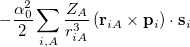
Calculations of spin-orbit couplings (SOCs) for TDDFT states within the Tamm-Dancoff approximation or RPA (including TDHF and CIS states) is available. We employ the one-electron Breit Pauli Hamiltonian to calculate the SOC constant between TDDFT states.
 |
 |
 |
(6.16) |
where  denotes electrons,
  denotes nuclei,
 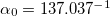 is the fine structure constant. Z
 is the bare positive charge on nucleus A. In the second quantization representation, the spin-orbit Hamiltonian in different directions can be expressed as
 |
|
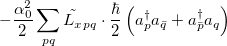 |
(6.17) | ||
 |
|
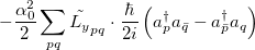 |
(6.18) | ||
 |
|
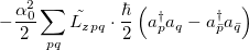 |
(6.19) |
where 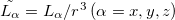 . The single-reference
  excited states (within the Tamm-Dancoff approximation) are given by
 |
|
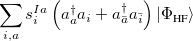 |
(6.20) | ||
 |
|
 |
(6.21) | ||
 |
|
 |
(6.22) | ||
 |
|
 |
(6.23) |
where  and
and  are singlet and triplet excitation coefficients of the
  singlet or triplet state respectively, with the normalization
  ;
;  refers to the Hartree-Fock ground state. Thus the SOC constant from the singlet state to different triplet manifolds can be obtained as follows,
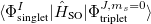 |
|
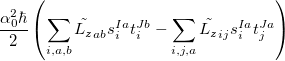 |
(6.24) | ||
 |
|
 |
|||
 |
 |
 |
(6.25) |
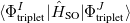
The SOC constant between different triplet manifolds can be obtained
 |
|
 |
|||
|
|
 |
(6.26) | ||
 |
|
 |
(6.27) |
Note that  . The total (root-mean-square) spin-orbit coupling is given by
 |
|
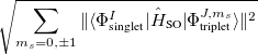 |
(6.28) | ||
 |
|
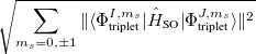 |
(6.29) |
For RPA states, the SOC constant can simply be obtained by replacing  (
( ) with
  (
( ) Setting the $rem variable CALC_SOC = TRUE will enable the SOC calculation for all calculated TDDFT states.
CALC_SOC
Controls whether to calculate the SOC constants for EOM-CC, ADC, and TDDFT within the TDA.
TYPE:
LOGICAL
DEFAULT:
FALSE
OPTIONS:
FALSE
Do not perform the SOC calculation.
TRUE
Perform the SOC calculation.
RECOMMENDATION:
None
Example 6.110 Calculation of SOCs for water molecule using TDDFT/B3LYP functional within the TDA.
$comment
   This sample input calculates the spin-orbit coupling constants for water
   between its ground state and its TDDFT/TDA excited triplets as well as the
   coupling between its TDDFT/TDA singlets and triplets.  Results are given in
   cm-1.
$end

$molecule
   0 1
   H       0.000000    -0.115747     1.133769
   H       0.000000     1.109931    -0.113383
   O       0.000000     0.005817    -0.020386
$end

$rem
   JOBTYPE              sp
   EXCHANGE             b3lyp
   BASIS                6-31G
   CIS_N_ROOTS          4
   CIS_CONVERGENCE      8
   CORRELATION          none
   MAX_SCF_CYCLES       600
   MAX_CIS_CYCLES       50
   SCF_ALGORITHM        diis
   MEM_STATIC           300
   MEM_TOTAL            2000
   SYMMETRY             false
   SYM_IGNORE           true
   UNRESTRICTED         false
   CIS_SINGLETS         true
   CIS_TRIPLETS         true
   CALC_SOC             true
   SET_ITER             300
$end
6.3.7 Various TDDFT-Based Examples
Example 6.111 This example shows two jobs which request variants of time-dependent density functional theory calculations. The first job, using the default value of RPA = FALSE, performs TDDFT in the Tamm-Dancoff approximation (TDA). The second job, with RPA = TRUE performs a both TDA and full TDDFT calculations.
$comment
   methyl peroxy radical
   TDDFT/TDA and full TDDFT with 6-31+G*
$end

$molecule
   0  2
   C  1.00412  -0.18045    0.00000
   O -0.24600   0.59615    0.00000
   O -1.31237  -0.23026    0.00000
   H  1.81077   0.56720    0.00000
   H  1.03665  -0.80545   -0.90480
   H  1.03665  -0.80545    0.90480
$end

$rem
   EXCHANGE          b
   CORRELATION       lyp
   CIS_N_ROOTS       5
   BASIS             6-31+G*
   SCF_CONVERGENCE   7
$end

@@@

$molecule
   read
$end

$rem
   EXCHANGE          b
   CORRELATION       lyp
   CIS_N_ROOTS       5
   RPA               true
   BASIS             6-31+G*
   SCF_CONVERGENCE   7
$end
Example 6.112 This example shows a calculation of the excited states of a formamide-water complex within a reduced excitation space of the orbitals located on formamide
$comment
   formamide-water TDDFT/TDA in reduced excitation space
$end

$molecule
   0 1
   H  1.13  0.49 -0.75
   C  0.31  0.50 -0.03
   N -0.28 -0.71  0.08
   H -1.09 -0.75  0.67
   H  0.23 -1.62 -0.22
   O -0.21  1.51  0.47
   O -2.69  1.94 -0.59
   H -2.59  2.08 -1.53
   H -1.83  1.63 -0.30
$end

$rem
   EXCHANGE          b3lyp
   CIS_N_ROOTS       10
   BASIS             6-31++G**
   TRNSS             TRUE
   TRTYPE            1
   CUTOCC            60
   CUTVIR            40
   CISTR_PRINT       TRUE
$end

$solute
1
2
3
4
5
6
$end
Example 6.113 This example shows a calculation of the core-excited states at the oxygen  -edge of CO with a short-range corrected functional.
$comment
   TDDFT with short-range corrected (SRC1) functional for the
   oxygen K-edge of CO
$end

$molecule
   0 1
   C     0.000000    0.000000   -0.648906
   O     0.000000    0.000000    0.486357
$end

$rem
   EXCHANGE       gen
   BASIS          6-311(2+,2+)G**
   CIS_N_ROOTS    6
   CIS_TRIPLETS   false
   TRNSS          true
   TRTYPE         3
   N_SOL          1
   SRC_DFT        1
   OMEGA          560
   OMEGA2         2450
   HF_SR          500
   HF_LR          170
$end

$solute
   1
$end

$xc_functional
   X  HF    1.00
   X  B     1.00
   C  LYP   0.81
   C  VWN   0.19
$end
Example 6.114 This example shows a calculation of the core-excited states at the phosphorus -edge with a short-range corrected functional.
$comment
   TDDFT with short-range corrected (SRC2) functional for the
   phosphorus K-edge of PH3
$end

$molecule
   0 1
   H     1.196206    0.000000   -0.469131
   P     0.000000    0.000000    0.303157
   H    -0.598103   -1.035945   -0.469131
   H    -0.598103    1.035945   -0.469131
$end

$rem
   EXCHANGE       gen
   BASIS          6-311(2+,2+)G**
   CIS_N_ROOTS    6
   CIS_TRIPLETS   false
   TRNSS          true
   TRTYPE         3
   N_SOL          1
   SRC_DFT        2
   OMEGA          2200
   OMEGA2         1800
   HF_SR          910
   HF_LR          280
$end

$solute
   1
$end

$xc_functional
   X  HF    1.00
   X  B     1.00
   C  LYP   0.81
   C  VWN   0.19
$end
Example 6.115 SF-TDDFT SP calculation of the 6 lowest states of the TMM diradical using recommended 50-50 functional
$molecule
   0 3
   C
   C  1  CC1
   C  1  CC2   2  A2
   C  1  CC2   2  A2     3  180.0
   H  2  C2H   1  C2CH   3    0.0
   H  2  C2H   1  C2CH   4    0.0
   H  3  C3Hu  1  C3CHu  2    0.0
   H  3  C3Hd  1  C3CHd  4    0.0
   H  4  C3Hu  1  C3CHu  2    0.0
   H  4  C3Hd  1  C3CHd  3    0.0

   CC1    = 1.35
   CC2    = 1.47
   C2H    = 1.083
   C3Hu   = 1.08
   C3Hd   = 1.08
   C2CH   = 121.2
   C3CHu  = 120.3
   C3CHd  = 121.3
   A2    = 121.0
$end

$rem
   EXCHANGE          gen
   BASIS             6-31G*
   SCF_GUESS         core
   SCF_CONVERGENCE   10
   MAX_SCF_CYCLES    100
   SPIN_FLIP         1
   CIS_N_ROOTS       6
   CIS_CONVERGENCE   10
   MAX_CIS_CYCLES    100
$end

$xc_functional
   X  HF    0.50
   X  S     0.08
   X  B     0.42
   C  VWN   0.19
   C  LYP   0.81
$end
Example 6.116 SF-DFT with non-collinear exchange-correlation functional for low-lying states of 
$comment
  Non-collinear SF-DFT calculation for CH2 at 3B1 state geometry from
  EOM-CCSD(fT) calculation
$end

$molecule
   0 3
   C
   H  1 rCH
   H  1 rCH  2 HCH

   rCH = 1.0775
   HCH = 133.29
$end

$rem
   EXCHANGE             PBE0
   BASIS                cc-pVTZ
   SPIN_FLIP            1
   WANG_ZIEGLER_KERNEL  TRUE
   SCF_CONVERGENCE      10
   CIS_N_ROOTS          6
   CIS_CONVERGENCE      10
$end