5.2 Møller-Plesset Perturbation Theory

5.2.1 Introduction

Møller-Plesset Perturbation Theory [128] is a widely used method for approximating the correlation energy of molecules. In particular, second order Møller-Plesset perturbation theory (MP2) is one of the simplest and most useful levels of theory beyond the Hartree-Fock approximation. Conventional and local MP2 methods available in Q-Chem are discussed in detail in Sections 5.3 and 5.4 respectively. The MP3 method is still occasionally used, while MP4 calculations are quite commonly employed as part of the G2 and G3 thermochemical methods [202, 203]. In the remainder of this section, the theoretical basis of Møller-Plesset theory is reviewed.

5.2.2 Theoretical Background

The Hartree-Fock wavefunction $\Psi _0$ and energy $E_0$ are approximate solutions (eigenfunction and eigenvalue) to the exact Hamiltonian eigenvalue problem or Schrödinger’s electronic wave equation, Eq. (4.5). The HF wavefunction and energy are, however, exact solutions for the Hartree-Fock Hamiltonian $H_{0}$ eigenvalue problem. If we assume that the Hartree-Fock wavefunction $\Psi _0$ and energy $E_0$ lie near the exact wave function $\Psi$ and energy $E$ , we can now write the exact Hamiltonian operator as

$\begin{equation} \label{eq500} H=H_0 +\lambda V \end{equation}$

(5.1)

where $V$ is the small perturbation and $\lambda$ is a dimensionless parameter. Expanding the exact wavefunction and energy in terms of the HF wavefunction and energy yields

$\begin{equation} \label{eq501} E=E^{(0)}+\lambda E^{(1)}+\lambda ^2E^{(2)}+\lambda ^3E^{(3)}+\ldots \end{equation}$

(5.2)

and

$\begin{equation} \label{eq02} \Psi =\Psi _0 +\lambda \Psi ^{(1)}+\lambda ^2\Psi ^{(2)}+\lambda ^3\Psi ^{(3)}+\ldots \end{equation}$

(5.3)

Substituting these expansions into the Schrödinger equation and collecting terms according to powers of $\lambda$ yields

$\begin{equation} \label{eq503} H_0 \Psi _0 =E^{(0)}\Psi _0 \end{equation}$

(5.4)

$\begin{equation} \label{eq504} H_0 \Psi ^{(1)}+V\Psi _0 =E^{(0)}\Psi ^{(1)}+E^{(1)}\Psi _0 \end{equation}$

(5.5)

$\begin{equation} \label{eq505} H_0 \Psi ^{(2)}+V\Psi ^{(1)}=E^{(0)}\Psi ^{(2)}+E^{(1)}\Psi ^{(1)}+E^{(2)}\Psi _0 \end{equation}$

(5.6)

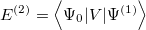
and so forth. Multiplying each of the above equations by $\Psi _0$ and integrating over all space yields the following expression for the $n$ th-order (MP $n$ ) energy:

$\begin{equation} \label{eq506} E^{(0)}=\langle {\Psi _0 } |H_0 | {\Psi _0 }\rangle \end{equation}$

(5.7)

$\begin{equation} \label{eq507} E^{(1)}=\langle {\Psi _0 } |V| {\Psi _0 }\rangle \end{equation}$

(5.8)

$\begin{equation} \label{eq508} E^{(2)}=\left\langle {\Psi _0 } |V| {\Psi ^{(1)}} \right\rangle \end{equation}$

(5.9)

Thus, the Hartree-Fock energy

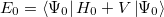$\begin{equation} \label{eq509} E_0 =\left\langle {\Psi _0 } \right|H_0 +V\left| {\Psi _0 } \right\rangle \end{equation}$

(5.10)

is simply the sum of the zeroth- and first- order energies

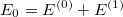$\begin{equation} \label{eq510} E_0 =E^{(0)}+E^{(1)} \end{equation}$

(5.11)

The correlation energy can then be written

$\begin{equation} \label{eq511} E_{\ensuremath{\mathrm{corr}}} =E_0^{(2)} +E_0^{(3)} +E_0^{(4)} +\ldots \end{equation}$

(5.12)

of which the first term is the MP2 energy.

It can be shown that the MP2 energy can be written (in terms of spin-orbitals) as

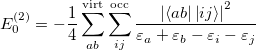$\begin{equation} \label{eq512} E_0^{(2)} =-\frac{1}{4}\sum _{ab}^{\ensuremath{\mathrm{virt}}} {\sum _{ij}^{\ensuremath{\mathrm{occ}}} {\frac{\left| {\left\langle {ab} \right|\left| {ij} \right\rangle } \right|^2}{\varepsilon _ a +\varepsilon _ b -\varepsilon _ i -\varepsilon _ j }} } \end{equation}$

(5.13)

where

$\begin{equation} \label{eq513} \left\langle {ab\left\| {ij} \right.} \right\rangle =\left\langle {ab} {\left| { {{ab} {ij}}} \right. \kern -}\nulldelimiterspace0.0pt{ij} \right\rangle -\left\langle {ab} {\left| { {{ab} {ji}}} \right. \kern -}\nulldelimiterspace0.0pt{ji} \right\rangle \end{equation}$

(5.14)

and

$\begin{equation} \label{eq514} \left\langle {ab} {\left| { {{ab} {cd}}} \right. \kern -}\nulldelimiterspace0.0pt{cd} \right\rangle =\int {\psi _ a ({\rm {\bf r}}_{\rm 1} )\psi _ c ({\rm {\bf r}}_{\rm 1} )\left[ {\frac{1}{r_{12} }} \right]\psi _ b ({\rm {\bf r}}_{\rm 2} )\psi _ d ({\rm {\bf r}}_{\rm 2} )d{\rm {\bf r}}_{\rm 1} d{\rm {\bf r}}_{\rm 2} } \end{equation}$

(5.15)

which can be written in terms of the two-electron repulsion integrals

$\begin{equation} \label{eq515} \left\langle {ab} {\left| {{{ab} {cd}}} \right. \kern -}\nulldelimiterspace0.0pt{cd} \right\rangle =\sum _\mu {\sum _\nu {\sum _\lambda {\sum _\sigma {C_{\mu a} C_{\nu c} C_{\lambda b} C_{\sigma d} \left( {\mu \nu \vert \lambda \sigma } \right)} } } } \end{equation}$

(5.16)

Expressions for higher order terms follow similarly, although with much greater algebraic and computational complexity. MP3 and particularly MP4 (the third and fourth order contributions to the correlation energy) are both occasionally used, although they are increasingly supplanted by the coupled-cluster methods described in the following sections. The disk and memory requirements for MP3 are similar to the self-consistent pair correlation methods discussed in Section 5.7 while the computational cost of MP4 is similar to the “(T)” corrections discussed in Section 5.8.