11.5 Effective Fragment Potential Method
The Effective Fragment Potential (EFP) method is a computationally inexpensive way of modeling intermolecular interactions in non-covalently bound systems. The EFP approach can be viewed as a QM/MM scheme with no empirical parameters. Originally EFP was developed by Gordon’s group [813, 814], and was implemented in GAMESS [815]. A review of the EFP theory and applications can be found in Ref. Ghosh:2010,Gordon:2012. A related approach, also based on distributed multipoles, is called XPol; it is described in Section 12.9.
A new implementation of the EFP method based on the libefp library (see http://www.libefp.org) has been added to Q-Chem.[818] The new EFP module is called EFPMAN2. EFPMAN2 can run calculations in parallel on a shared memory multi-core computer and is much faster than the previous EFP implementation in Q-Chem. EFPMAN2 is interfaced with CCMAN and CCMAN2 modules to allow coupled cluster and EOM-CC calculations with EFP. CIS and TDDFT calculations with EFP are also available.
11.5.1 Theoretical Background
The total energy of the system consists of the interaction energy of the effective fragments ( ) and the energy of the ab initio (i.e., QM) region in the field of the fragments. The former includes electrostatics, polarization, dispersion and exchange-repulsion contributions (the charge-transfer term, which might be important for description of the ionic and highly polar species, is omitted in the current implementation):
 |
(11.58) |
The QM-EF interactions are computed as follows. The electrostatics and polarization parts of the EFP potential contribute to the quantum Hamiltonian via one-electron terms,
 |
(11.59) |
whereas dispersion and exchange-repulsion QM-EF interactions are treated as additive corrections to the total energy.
The electrostatic component of the EFP energy accounts for Coulomb interactions. In molecular systems with hydrogen bonds or polar molecules, this is the leading contribution to the total inter-molecular interaction energy [819]. An accurate representation of the electrostatic potential is achieved by using multipole expansion (obtained from the Stone’s distributed multipole analysis) around atomic centers and bond midpoints (i.e., the points with high electronic density) and truncating this expansion at octupoles [634, 635, 813, 814]. The fragment-fragment electrostatic interactions consist of charge-charge, charge-dipole, charge-quadrupole, charge-octupole, dipole-dipole, dipole-quadrupole, and quadrupole-quadrupole terms, as well as terms describing interactions of electronic multipoles with the nuclei and nuclear repulsion energy.
Electrostatic interaction between an effective fragment and the QM part is described by perturbation  of the ab initio Hamiltonian (see Eq. (11.59)). The perturbation enters the one-electron part of the Hamiltonian as a sum of contributions from the expansion points of the effective fragments. Contribution from each expansion point consists of four terms originating from the electrostatic potential of the corresponding multipole (charge, dipole, quadrupole, and octupole).
The multipole representation of the electrostatic density of a fragment breaks down when the fragments are too close. The multipole interactions become too repulsive due to significant overlap of the electronic densities and the charge-penetration effect. The magnitude of the charge-penetration effect is usually around 15% of the total electrostatic energy in polar systems, however, it can be as large as 200% in systems with weak electrostatic interactions [820]. To account for the charge-penetration effect, the simple exponential damping of the charge-charge term is used [821, 820]. The charge-charge screened energy between the expansion points  and
and  is given by the following expression, where
  and
and  are the damping parameters associated with the corresponding expansion points:
 |
 |
![$\displaystyle \left[ 1 - (1 + \alpha _ k R_{kl}/2) e^{-\alpha _ k R_{kl}} \right] q^ k q^ l/R_{kl} \; \; \; ,~ ~ \mbox{if $\alpha _ k=\alpha _ l$} $](images/img-2116.png) |
(11.60) | ||
 |
|
 |
Damping parameters are included in the potential of each fragment, but QM-EFP electrostatic interactions are currently calculated without damping corrections.
Alternatively, one can obtain the short-range charge-penetration energy using the spherical Gaussian overlap (SGO) approximation [822]:
 |
(11.61) |
where  is the overlap integral between localized MOs and (calculated for the exchange-repulsion term, Eq. ()). This charge-penetration energy is calculated and printed separately from the rest of the electrostatic energy. Using overlap-based damping generally results in a more balanced description of intermolecular interactions and is recommended.
Polarization accounts for the intramolecular charge redistribution in response to external electric field. It is the major component of many-body interactions responsible for cooperative molecular behavior. EFP employs distributed polarizabilities placed at the centers of valence LMOs. Unlike the isotropic total molecular polarizability tensor, the distributed polarizability tensors are anisotropic.
The polarization energy of a system consisting of an ab initio and effective fragment regions is computed as [813]
 |
(11.62) |
where  and
and  are the induced dipole and the conjugated induced dipole at the distributed point ;
  is the external field due to static multipoles and nuclei of other fragments, and
  and
and  are the fields due to the electronic density and nuclei of the ab initio part, respectively.
The induced dipoles at each polarizability point are computed as
 |
(11.63) |
where  is the distributed polarizability tensor at . The total field
  comprises from the static field and the field due to other induced dipoles,
  , as well as the field due to nuclei and electronic density of the ab initio region:
 |
(11.64) |
As follows from the above equation, the induced dipoles on a particular fragment depend on the values of the induced dipoles of all other fragments. Moreover, the induced dipoles on the effective fragments depend on the ab initio electronic density, which, in turn, is affected by the field created by these induced dipoles through a one electron contribution to the Hamiltonian:
 |
(11.65) |
where  and
and  are the distance and its Cartesian components between an electron and the polarizability point . In sum, the total polarization energy is computed self-consistently using a two level iterative procedure. The objectives of the higher and lower levels are to converge the wave function and induced dipoles for a given fixed wave function, respectively. In the absence of the ab initio region, the induced dipoles of the EF system are iterated until self-consistent with each other.
Self-consistent treatment of polarization accounts for many-body interaction effects. Polarization energy between EFP fragments is augmented by gaussian-like damping functions with default parameter  , applied to electric field
  [822]:
 |
(11.66) |
 |
(11.67) |
Dispersion provides a leading contribution to van der Waals and  -stacking interactions. The dispersion interaction is expressed as the inverse dependence:
 |
(11.68) |
where coefficients  are derived from the frequency-dependent distributed polarizabilities with expansion points located at the LMO centroids, i.e., at the same centers as the polarization expansion points. The higher-order dispersion terms (induced dipole-induced quadrupole, induced quadrupole/induced quadrupole, etc.) are approximated as
  of the term [823].
For small distances between effective fragments dispersion interactions are corrected for charge penetration and electronic density overlap effect either with the Tang-Toennies damping formula [824] with parameter  :
:
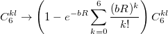 |
(11.69) |
or using interfragment overlap (so called overlap-based damping)[822]:
 |
(11.70) |
QM-EFP dispersion interactions are currently disabled.
Exchange-repulsion originates from the Pauli exclusion principle, which states that the wave function of two identical fermions must be anti-symmetric. In traditional classical force fields, exchange-repulsion is introduced as a positive (repulsive) term, e.g.,  in the Lennard-Jones potential. In contrast, EFP uses a wave function-based formalism to account for this inherently quantum effect. Exchange-repulsion is the only non-classical component of EFP and the only one that is repulsive.
The exchange-repulsion interaction is derived as an expansion in the intermolecular overlap, truncated at the quadratic term [825, 826], which requires that each effective fragment carries a basis set that is used to calculate overlap and kinetic one-electron integrals for each interacting pair of fragments. The exchange-repulsion contribution from each pair of localized orbitals  and
and  belonging to fragments
  and
and  , respectively, is:
 |
|
 |
(11.71) | ||
 |
|
 |
|||
|
|
 |
where , , and are the LMOs,  and
and  are the nuclei,
  and
and  are the intermolecular overlap and kinetic energy integrals, and is the Fock matrix element.
The expression for the  involves overlap and kinetic energy integrals between pairs of localized orbitals. In addition, since Eq. eq:ex_rep is derived within an infinite basis set approximation, it requires a reasonably large basis set to be accurate [6-31+G* is considered to be the smallest acceptable basis set, 6-311++G(3df,2p) is recommended]. These factors make exchange-repulsion the most computationally expensive part of the EFP energy calculations of moderately sized systems.
Large systems require additional considerations. Since total exchange-repulsion energy is given by a sum of terms in Eq. () over all the fragment pairs, its computational cost formally scales as  with the number of effective fragments
  . However, exchange-repulsion is a short-range interaction; the overlap and kinetic energy integrals decay exponentially with the inter-fragment distance. Therefore, by employing a distance-based screening, the number of overlap and kinetic energy integrals scales as
  . Consequently, for large systems exchange-repulsion may become less computationally expensive than the long-range components of EFP (such as Coulomb interactions).
The QM-EFP exchange-repulsion energy is currently disabled.
11.5.2 Excited-State Calculations with EFP
Interface of EFP with EOM-CCSD (both via CCMAN and CCMAN2), CIS, CIS(D), and TDDFT has been developed [827, 828]. In the EOM-CCSD/EFP calculations, the reference-state CCSD equations for the cluster amplitudes are solved with the HF Hamiltonian modified by the electrostatic and polarization contributions due to the effective fragments, Eq. (11.59). In the coupled-cluster calculation, the induced dipoles of the fragments are frozen at their HF values.
The transformed Hamiltonian  effectively includes Coulomb and polarization contributions from the EFP part. As is diagonalized in an EOM calculation, the induced dipoles of the effective fragments are frozen at their reference state value, i.e., the EOM equations are solved with a constant response of the EFP environment. To account for solvent response to electron rearrangement in the EOM target states (i.e., excitation or ionization), a perturbative non-iterative correction is computed for each EOM root as follows. The one-electron density of the target EOM state (excited or ionized) is calculated and used to re-polarize the environment, i.e., to recalculate the induced dipoles of the EFP part in the field of an EOM state. These dipoles are used to compute the polarization energy corresponding to this state.
The total energy of the excited state with inclusion of the perturbative response of the EFP polarization is:
 |
(11.72) |
where  is the energy found from EOM-CCSD procedure and
  has the following form:
 |
 |
 |
(11.73) | ||
|
 |
![$\displaystyle + (\tilde{\mu }_{\mathrm{ex},a}^ k F_{\mathrm{ex},a}^{\mathrm{ai},k} - \tilde{\mu }_{\mathrm{gr},a}^ k F_{\mathrm{gr},a}^{\mathrm{ai},k}) - (\mu _{\mathrm{ex},a}^ k - \mu _{\mathrm{gr},a}^ k + \tilde{\mu }_{\mathrm{ex},a}^ k - \tilde{\mu }_{\mathrm{gr},a}^ k) F_{\mathrm{ex},a}^{\mathrm{ai},k}\Bigr ] \nonumber $](images/img-2155.png) |
where  and
and  are the fields due to the reference (HF) state and excited-state electronic densities, respectively.
  and
and  are the induced dipole and conjugated induced dipole at the distributed polarizability point consistent with the reference-state density, while
  and
and  are the induced dipoles corresponding to the excited state density.
The first two terms in Eq. (11.73) provide a difference of the polarization energy of the QM/EFP system in the excited and ground electronic states; the last term is the leading correction to the interaction of the ground-state-optimized induced dipoles with the wave function of the excited state.
The EOM states have both direct and indirect polarization contributions. The indirect term comes from the orbital relaxation of the solute in the field due to induced dipoles of the solvent. The direct term given by Eq. (11.73) is the response of the polarizable environment to the change in solute’s electronic density upon excitation. Note that the direct polarization contribution can be very large (tenths of eV) in EOM-IP/EFP since the electronic densities of the neutral and the ionized species are very different.
An important advantage of the perturbative EOM/EFP scheme is that it does not compromise multi-state nature of EOM and that the electronic wave functions of the target states remain orthogonal to each other since they are obtained with the same (reference-state) field of the polarizable environment. For example, transition properties between these states can be calculated.
EOM-CC/EFP scheme works with any type of the EOM excitation operator  currently supported in Q-Chem, i.e., spin-flipping (SF), excitation energies (EE), ionization potential (IP), electron affinity (EA) (see Section 6.7.12 for details). However, direct polarization correction requires calculation of one-electron density of the excited state, and will be computed only for the methods with implemented one-electron properties.
Implementation of CIS/EFP, CIS(D)/EFP, and TDDFT/EFP methods is similar to the implementation of EOM/EFP. Polarization correction as in Eq. 11.73 is calculated and added to the CIS or TDDFT excitation energies.
11.5.3 Extension to Macromolecules: Fragmented EFP Scheme
Macromolecules such as proteins or DNA present a large number of electronic structure problems (photochemistry, redox chemistry, reactivity) that can be described within QM/EFP framework. EFP has been extended to deal with such complex systems via the so-called fragmented EFP scheme (fEFP). The current Q-Chem implementation allows one to (i) compute interaction energy between a ligand and a macromolecule (both represented by EFP) and (ii) to calculate the excitation energies, ionization potentials, electronic affinities of a QM moiety interacting with a fEFP macromolecule using QM/EFP scheme (see Section 11.5.2). In the present implementation, the ligand cannot be covalently bound to the macromolecule.
There are multiple ways to cut a large molecule into units depending on the position of the cut between two covalently bound residues. An obvious way to cut a protein is to cut through peptide bonds such that each fragment represents one amino acid. Alternatively, one can cut bonds between two atoms of the same nature (carbonyl and carbon- or carbon- and the first carbon of the side chain). The user can choose the most appropriate way to cut.
Consider a protein ( ) consisting of amino acids,
  , and is split into fragments (
 ). The fragments can be saturated by either Hydrogen Link Atom[795] (HLA) or by mono-valent groups of atoms from the neighboring fragment(s) called hereafter Cap Link Atom (CLA). If fragments are capped using the HLA scheme, the hydrogen is located along the peptide bond axis and at the distance corresponding to the equilibrium bond length of a CH bond:
 |
(11.74) |
In the CLA scheme, the cap has exactly the same geometry as the respective neighboring group. If the cuts are made through peptide bonds (one fragment is one amino acid), the caps ( ) are either an aldehyde to saturate the -N(H) end of the fragment, or an amine to saturate the -C(=O) extremity of the fragment.
 |
(11.75) |
Q-Chem provides a two-step script, prefefp.pl, located in $QC/bin which takes a PDB file and breaks it into capped fragments in the GAMESS format, such that the EFP parameters for these capped fragments can be generated, as explained in Section 11.5.7. As the EFP parameters are generated for each capped fragment, the neighboring fragments have duplicated parameter points (overlapping areas) in both the HLA and CLA schemes due to the overlapping caps. Since multipole expansion points and polarizability expansion points are computed on each capped residue by the standard procedure, the multipole (and damping terms) and polarizabilities need to be removed ( ) from the overlapping areas.
Equations (11.74) and (11.75) become:
 |
(11.76) |
The details concerning this removing procedure are presented in Section 11.5.7.
Once these duplicate parameters are removed from the EFP parameters of the capped fragments, the EFP-EFP and QM-EFP calculations can be conducted as usual.
Currently, fEFP includes electrostatic and polarization contributions, which appear in EFP(ligand)/fEFP(macromolecule) and in QM/fEFP calculations (note that the QM part is not covalently bound to the macromolecule). Consequently, the total interaction energy ( ) between a ligand (
 ) and a protein () divided into fragments is:
 |
(11.77) |
The electrostatics is an additive term; its contribution to fragment-fragment and ligand-fragment interaction is computed as follows:
 |
(11.78) |
The polarization contribution in an EFP system (no QM) is:
 |
(11.79) |
The first term is the polarization energy obtained upon convergence of the induced dipoles of the ligand ( ) and all fragments (
 ). The system is thus fully polarized, all fragments (A
 or L) are polarizing each other until self-consistency.
 |
 |
|||
 |
 |
(11.80) |
The second term of Eq. (11.79) is the polarization of the protein by itself; this value has to be subtracted once the induced dipoles (Eq. 11.80) converged.
The LA scheme is available to perform QM/fEFP job. In this situation the fEFP has to include a macromolecule (covalent bond between fragments). This scheme is not able yet to perform QM/fEFP/EFP in which a macromolecule and solvent molecules would be described at the EFP level of theory.
In addition to the HLA and CLA schemes, Q-Chem also features Molecular Fragmentation with Conjugated Caps approach (MFCC) which avoids the issue of overlapping of saturated fragments and was developed in 2003 by Zhang[829, 830]. MFCC procedure consists of a summation over the interactions between a ligand and capped residues (CLA scheme) and a subtraction over the interactions of merged caps ( ), the so-called “concaps”, with the ligand.
  concap fragments are actually used to subtract the overlapping effect.
 |
(11.81) |
In this scheme the contributions due to overlapping caps simply cancel out and the EFP parameters do not need any modifications, in contrast to the HLA or CLA procedures. However, the number of parameters that need to be generated is larger ( capped fragments + concaps).
The MFCC electrostatic interaction energy is given as the sum of the interaction energy between each capped fragment ( ) and the ligand minus the interaction energy between each concap (
 ) and the ligand:
 |
(11.82) |
The main advantage of MFCC is that the multipole expansion obtained on each capped residue or concap are kept during the  calculation. In the present implementation, there are no polarization contributions. The MFCC scheme is not yet available for QM/fEFP.
11.5.4 Running EFP Jobs
The current version supports single point calculations in systems consisting of () ab initio and EFP regions (QM/MM); or ( ) EFP region only. The ab initio region can be described by conventional quantum methods like HF, DFT, or correlated methods including methods for the excited states [CIS, CIS(D), TDDFT, EOM-CCSD methods]. Theoretical details on the interface of EFP with EOM-CCSD and CIS(D) can be found in Refs. Slipchenko:2010,Kosenkov:2011.
Note: EFP provides both implicit (through orbital response) and explicit (as instantaneous response of the polarizable EFP fragments) corrections to the electronic excited states. EFP-modified excitation energies are printed in the property section of the output.
Electrostatic, polarization, exchange-repulsion, and dispersion contributions are calculated between EFs; only electrostatic and polarization terms are evaluated between ab initio and EF regions.
The ab initio region is specified by regular Q-Chem input using $molecule and $rem sections. In calculations with no QM part, the $molecule section should contain a dummy atom (for example, helium).
Positions of EFs are specified in the $efp_fragments section. Two geometry formats are available for fragments, Euler angle format and XYZ format. In Euler angle format, each line in this section contains the information on an individual fragment: fragment’s name and position, specified by center-of-mass coordinates ( ,
,  ,
,  ) and the Euler rotation angles (,
  ,
,  ) relative to the fragment frame, i.e., the coordinates of the standard fragment provided in the fragment library. The XYZ format is identical to the coordinate format used in GAMESS; i.e., the name of the fragment is provided on the first line followed by three lines specifying names and x,y,z coordinates of first three atoms of the fragment.
When using EFPMAN2 you can also specify positions and orientations of the fragments using (, , ) coordinates of the first three atoms of the fragment. To enable this feature use EFP_COORD_XYZ keyword. The format of input goes as follows: for each fragment the first line should contain the name of the fragment and the following three lines should specify coordinates of the three first atoms belonging to a fragment. The sample input can be found in the examples section below.
11.5.5 Library of Fragments
The effective fragments are rigid and their potentials are generated from a set of ab initio calculations on each unique isolated fragment. The EFP includes: () multipoles (produced by the Stone’s Distributed Multipolar Analysis) for Coulomb and polarization terms; () static polarizability tensors centered at localized molecular orbital (LMO) centroids (obtained from coupled-perturbed Hartree-Fock calculations), which are used for calculations of polarization; ( ) dynamic polarizability tensors centered on the LMOs that are generated by time-dependent HF calculations and used for calculations of dispersion; and (
 ) the Fock matrix, basis set, and localized orbitals needed for the exchange-repulsion term. Additionally, the EF potential contains coordinates of atoms, coordinates of the points of multi-polar expansion (typically, atoms and bond mid-points), coordinates of the LMO centroids, electrostatic and polarization screening parameters, and atomic labels of the EF atoms.
Q-Chem provides a library of standard fragments with precomputed effective fragment potentials. Currently the library includes common organic solvents, nucleobases, and molecules from S22 and S66 datasets for non-covalent interactions; see Table 11.6. EFP potentials in GAMESS format are supported by new EFPMAN2 module. They are stored in $QCAUX/fraglib directory.
acetone |
ACETONE_L |
acetonitrile |
ACETONITRILE_L |
adenine |
ADENINE_L |
ammonia |
AMMONIA_L |
benzene |
BENZENE_L |
carbon tetrachloride |
CCL4_L |
cytosine C1 |
CYTOSINE_C1_L |
cytosine C2a |
CYTOSINE_C2A_L |
cytosine C2b |
CYTOSINE_C2B_L |
cytosine C3a |
CYTOSINE_C3A_L |
cytosine C3b |
CYTOSINE_C3B_L |
dichloromethane |
DCM_L |
dimethyl sulfoxide |
DMSO_L |
guanine enol N7 |
GUANINE_EN7_L |
guanine enol N9 |
GUANINE_EN9_L |
guanine enol N9RN7 |
GUANINE_EN9RN7_L |
guanine keton N7 |
GUANINE_KN7_L |
guanine keton N9 |
GUANINE_KN9_L |
methane |
METHANE_L |
methanol |
METHANOL_L |
phenol |
PHENOL_L |
thymine |
THYMINE_L |
toluene |
TOLUENE_L |
water |
WATER_L |
acetamide, S66, gas phase |
ACETAMIDE_L |
acetamide, S66, H-bonded dimer |
ACETAMIDE_HB_L |
acetic acid, S66, gas phase |
ACETICAC_L |
acetic acid, S66, H-bonded dimer |
ACETICAC_HB_L |
adenine, S22 stack dimer |
ADENINE_L |
adenine, S22 WC dimer |
ADENINE_WC_L |
2-aminopyridine, S22 |
AMINOPYRIDINE_L |
cyclopentane, S66 |
CPENTANE_L |
ethylene |
ETHENE_L |
acetylene |
ETHYNE_L |
formic acid, S22 H-bonded dimer |
FORMICAC_HB_L |
formamide, S22 dimer |
FORMID_L |
hydrogen cyanide |
HCN_L |
indole, S22 |
INDOLE_L |
methylamine, S66 |
MENH2_L |
neopentane, S66 |
NEOPENTANE_L |
|
O2_L |
pentane, S66 |
PENTANE_L |
peptide, S66 |
PEPTIDE_L |
pyrazine |
PYRAZINE_L |
pyridine, S66 |
PYRIDINE_L |
2-pyridoxine, S22 |
PYRIDOXINE_L |
thymine, S22 stack dimer |
THYMINE_L |
thymine, S22 WC dimer |
THYMINE_WC_L |
uracil, S66, gas phase |
URACIL_L |
uracil, S66, H-bonded dimer |
URACIL_HB_L |

Note: The fragments from Q-Chem fragment library have _L added to their names to distinguish them from user-defined fragments.
The parameters for the standard fragments were computed as follows. The geometries of the solvent molecules were optimized by MP2/cc-pVTZ; geometries of nucleobases were optimized with RI-MP2/cc-pVTZ. Geometries of molecules from S22 and S66 datasets are discussed in Ref.Flick:2012. The EFP parameters were obtained in GAMESS. To generate the electrostatic multipoles and electrostatic screening parameters, analytic DMA procedure was used, with 6-31+G* basis for non-aromatic compounds and 6-31G* for aromatic compounds and nucleobases. The rest of the potential, i.e., static and dynamic polarizability tensors, wave function, Fock matrix, etc., were obtained using 6-311++G(3df,2p) basis set.
11.5.6 Calculation of User-Defined EFP Potentials
User-defined EFP parameters can be generated in MAKEFP job in GAMESS (see the GAMESS manual for details).
The EFP potential generation begins by determining an accurate structure for the fragment (EFP is the frozen-geometry potential, so the fragment geometry will remain the same in all subsequent calculations). We recommend MP2/cc-PVTZ level of theory.
11.5.6.1 Generating EFP Parameters in GAMESS
EFP parameters can be generated in GAMESS using MAKEFP job (RUNTYP=MAKEFP). For EFP parameters calculations, 6-311++G(3df,2p) basis set is recommended. Original Stone’s distributed multipole analysis (bigexp=0 in the group $stone is recommended for non-aromatic compound; optionally, one may decrease the basis set to 6-31G* or 6-31+G* for generation of electrostatic multipoles and screening parameters. (To prepare such a “mixed" potential, one has to run two separate MAKEFP calculations in larger and smaller bases, and combine the corresponding parts of the potential). In aromatic compounds, one must either use numerical grid for generation of multipoles (bigexp=4.0) or use 6-31G* basis with standard analytic DMA, which is recommended. The MAKEFP job produces (usually in the scratch directory) the .efp file containing all the necessary EFP parameters. See GAMESS manual for further details. Below are examples of the RUNTYP=MAKEFP GAMESS input file for water and benzene.
GAMESS input example for water.

 $contrl units=angs local=boys runtyp=makefp coord=cart icut=11 $end
 $system timlim=99999 mwords=200 $end
 $scf soscf=.f. diis=.t. conv=1.0d-06 $end
 $basis gbasis=n311 ngauss=6 npfunc=2 ndfunc=3 nffunc=1
   diffs=.t. diffsp=.t. $end
 $stone
   bigexp=0.0
 $end
 $damp ifttyp(1)=3,2 iftfix(1)=1,1 thrsh=500.0 $end
 $dampgs
h3=h2
bo31=bo21
 $end
 $data
 water h2o (geometry: mp2/cc-pvtz)
 c1
o1 8.0 	0.0000 	0.0000  0.1187
h2 1.0	0.0000 	0.7532 -0.4749
h3 1.0	0.0000 -0.7532 -0.4749
 $end
GAMESS input example for benzene.

 $contrl units=bohr local=boys runtyp=makefp coord=cart icut=11 $end
 $system timlim=99999 mwords=200 $end
 $scf soscf=.f. diis=.t. conv=1.0d-06  $end
 $basis gbasis=n311 ngauss=6 npfunc=2 ndfunc=3 nffunc=1
   diffs=.t. diffsp=.t. $end
 $stone
   bigexp=4.0
 $end
 $damp ifttyp(1)=3,2 iftfix(1)=1,1 thrsh=500.0 $end
 $dampgs
c6=c5
c2=c1
c3=c1
c4=c1
c5=c1
c6=c1
h8=h7
h9=h7
h10=h7
h11=h7
h12=h7
bo32=bo21
bo43=bo21
bo54=bo21
bo61=bo21
bo65=bo21
bo82=bo71
bo93=bo71
bo104=bo71
bo115=bo71
bo126=bo71
 $end
 $data
benzene c6h6 (geometry: mp2/cc-pvtz)
c1
c1     6.0    1.3168      -2.2807       0.0000
c2     6.0    2.6336       0.0000       0.0000
c3     6.0    1.3168       2.2807       0.0000
c4     6.0   -1.3168       2.2807       0.0000
c5     6.0   -2.6336      -0.0000       0.0000
c6     6.0   -1.3168      -2.2807       0.0000
h7     1.0    2.3386      -4.0506       0.0000
h8     1.0    4.6772       0.0000       0.0000
h9     1.0    2.3386       4.0506       0.0000
h10    1.0   -2.3386       4.0506       0.0000
h11    1.0   -4.6772       0.0000       0.0000
h12    1.0   -2.3386      -4.0506       0.0000
 $end
11.5.7 fEFP Input Structure
A two-step script, prefefp.pl located in $QC/bin, allows users to break molecular structures from a PDB file into the capped fragments in the GAMESS format, such that parameters for fEFP calculations can be generated.
To use the prefefp.pl scripts you need a PDB file, a MAP file, and a directory with all your .efp parameter files. Run the following commands to: (1) obtain the input file generating the EFP parameters for the capped fragments, and (2) create the EFP input file in XYZ format.
perl prefp.pl 1 <PDB file> <MAP file>
perl prefp.pl 2 <PDB file> <.efp path> <MAP file> <GMS input file name>
At the first step the script splits the biomolecule (PDB format) into fragments generating GAMESS MAKEFP input files with the help of a MAP file.
At the second step the .efp file from GAMESS MAKEFP is analyzed and is auto-edited using the same MAP file to create the final EFP input (XYZ format).
The MAP file is required as an input for the script. It defines groups of atoms belonging to each EFP fragment both for the MAKEFP calculation and for the consequent EFP jobs. Here is a description of the MAP file: Each fragment described using section $RESIDUE followed by closing $end In this example the Lys2 is extracted cutting through the peptidic bond, the cut bond is saturated with hydrogen atom. The explanation of each variable is given below.
$Residue
Name = lys2
PreAtoms = 14-35
NH = 14,12
CH = 34,36
PostAtoms = 14-35
Rescharge = +1
USEFP = lys2
$end
The four first lines are required for the first step of the script (GAMESS MAKEFP job); the next ones are necessary for the actual EFP job.
Name: Residue name
PreAtoms: Atoms which belongs to the residue for GAMESS MAKEFP calculation.
CH, NH, or OH: In the case of broken bonds a hydrogen atom is added so that in X-Y bond (X belongs to the Lys2 residue and Y belongs to the previous or next residue) the Y atom is replaced by H along the X-Y axis. The default equilibrium distance for the X-H bond is set to 1.08 for a C-H bond, to 1.00 for a N-H bond, and to 0.94 for a O-H bond. It required to specify the atom number of the X and Y atoms.
PostAtoms: Atoms which belong to the residue after removing the overlapping fragment atoms or caps when the HLA or the CLA scheme is used. This important step removes multipoles and polarizability expansion points of those atoms according to the cutoff procedure (set by default to 1.3 and 1.2 for multipoles and polarizability expansion points, respectively). Multipole expansion at duplicated points are eliminated but to maintain the net integer charge on each amino acid the monopole expansion of the caps is redistributed on the natural fragment. This method is called Expand-Remove-Redistribute. Concerning the polarizability expansion points, only one polarizability expansion point is removed when a hydrogen atom saturates the dangling bond, whereas 6 or 5 polarizability points are removed when the cap is an amine or an aldehyde, respectively.
ResCharge: The net charge of the residue after removing the overlapping fragment atoms (cfr. LA scheme).
USEFP: Name of the EFP fragment (and .efp file) to use with this fragment in the actual EFP calculation.
Note: In the MFCC scheme, the two first letters of the concap fragment have to be ’CC’.
Note: If the PostAtoms keyword is not present, the second script will generate an EFP job file without any modification of the parameters, which is useful for the MFCC scheme.
11.5.8 Input keywords
EFP_COORD_XYZ
Use coordinates of three atoms instead of Euler angles to specify position and orientation of the fragments
TYPE:
LOGICAL
DEFAULT:
FALSE
OPTIONS:
TRUE FALSE
RECOMMENDATION:
None
EFP_DIRECT_POLARIZATION_DRIVER
Use direct solver for EFP polarization
TYPE:
LOGICAL
DEFAULT:
FALSE
OPTIONS:
TRUE FALSE
RECOMMENDATION:
Direct polarization solver provides stable convergence of induced dipoles which may otherwise become problematic in case of closely lying or highly polar or charged fragments. The computational cost of direct polarization versus iterative polarization becomes higher for systems containing more than 10000 polarizable points.
EFP_ENABLE_LINKS
Enable fragment links in EFP region
TYPE:
LOGICAL
DEFAULT:
FALSE
OPTIONS:
TRUE FALSE
RECOMMENDATION:
None
EFP
Specifies that EFP calculation is requested
TYPE:
LOGICAL
DEFAULT:
FALSE
OPTIONS:
TRUE FALSE
RECOMMENDATION:
The keyword should be present if excited state calculation is requested
EFP_FRAGMENTS_ONLY
Specifies whether there is a QM part
TYPE:
LOGICAL
DEFAULT:
FALSE
QM part is present
OPTIONS:
TRUE
Only MM part is present: all fragments are treated by EFP
FALSE
QM part is present: do QM/MM EFP calculation
RECOMMENDATION:
None
EFP_INPUT
Specifies the format of EFP input
TYPE:
LOGICAL
DEFAULT:
FALSE
Dummy atom (e.g., He) in $molecule section should be present
OPTIONS:
TRUE
A format without dummy atom in $molecule section
FALSE
A format with dummy atom in $molecule section
RECOMMENDATION:
None
FEFP_EFP
Specifies that fEFP_EFP calculation is requested to compute the total interaction energies between a ligand (the last fragment in the $efp_fragments section) and the protein (represented by fEFP)
TYPE:
STRING
DEFAULT:
OFF
OPTIONS:
OFF
disables fEFP
LA
enables fEFP with the Link Atom (HLA or CLA) scheme (only electrostatics and polarization)
MFCC
enables fEFP with MFCC (only electrostatics)
RECOMMENDATION:
The keyword should be invoked if EFP/fEFP is requested (interaction energy calculations). This keyword has to be employed with EFP_FRAGMENT_ONLY = TRUE. To switch on/off electrostatics or polarzation interactions, the usual EFP controls are employed.
FEFP_QM
Specifies that fEFP_QM calculation is requested to perform a QM/fEFPcompute computation. The fEFP part is a fractionated macromolecule.
TYPE:
STRING
DEFAULT:
OFF
OPTIONS:
OFF
disables fEFP_QM and performs a QM/EFP calculation
LA
enables fEFP_QM with the Link Atom scheme
RECOMMENDATION:
The keyword should be invoked if QM/fEFP is requested. This keyword has to be employed with efp_fragment_only false. Only electrostatics is available.
EFP_ELEC
Controls fragment-fragment electrostatics in EFP
TYPE:
LOGICAL
DEFAULT:
TRUE
OPTIONS:
TRUE
switch on electrostatics
FALSE
switch off electrostatics
RECOMMENDATION:
None
EFP_POL
Controls fragment-fragment polarization in EFP
TYPE:
LOGICAL
DEFAULT:
TRUE
OPTIONS:
TRUE
switch on polarization
FALSE
switch off polarization
RECOMMENDATION:
None
EFP_DISP
Controls fragment-fragment dispersion in EFP
TYPE:
LOGICAL
DEFAULT:
TRUE
OPTIONS:
TRUE
switch on dispersion
FALSE
switch off dispersion
RECOMMENDATION:
None
EFP_EXREP
Controls fragment-fragment exchange repulsion in EFP
TYPE:
LOGICAL
DEFAULT:
TRUE
OPTIONS:
TRUE
switch on exchange repulsion
FALSE
switch off exchange repulsion
RECOMMENDATION:
None
EFP_QM_ELEC
Controls QM-EFP electrostatics
TYPE:
LOGICAL
DEFAULT:
TRUE
OPTIONS:
TRUE
switch on QM-EFP electrostatics
FALSE
switch off QM-EFP electrostatics
RECOMMENDATION:
None
EFP_QM_POL
Controls QM-EFP polarization
TYPE:
LOGICAL
DEFAULT:
TRUE
OPTIONS:
TRUE
switch on QM-EFP polarization
FALSE
switch off QM-EFP polarization
RECOMMENDATION:
None
EFP_QM_DISP
Controls QM-EFP dispersion
TYPE:
LOGICAL
DEFAULT:
FALSE
OPTIONS:
TRUE
switch on QM-EFP dispersion
FALSE
switch off QM-EFP dispersion
RECOMMENDATION:
None
EFP_QM_EXREP
Controls QM-EFP exchange-repulsion
TYPE:
LOGICAL
DEFAULT:
FALSE
OPTIONS:
TRUE
switch on QM-EFP exchange-repulsion
FALSE
switch off QM-EFP exchange-repulsion
RECOMMENDATION:
None
EFP_ELEC_DAMP
Controls fragment-fragment electrostatic screening in EFP
TYPE:
INTEGER
DEFAULT:
2
OPTIONS:
0
switch off electrostatic screening
1
use overlap-based damping correction
2
use exponential damping correction if screening parameters are provided in the EFP potential
RECOMMENDATION:
Overlap-based damping is recommended
EFP_DISP_DAMP
Controls fragment-fragment dispersion screening in EFP
TYPE:
INTEGER
DEFAULT:
2
OPTIONS:
0
switch off dispersion screening
1
use Tang-Toennies screening, with fixed parameter
2
use overlap-based damping
RECOMMENDATION:
None
EFP_POL_DAMP
Controls fragment-fragment polarization screening in EFP
TYPE:
INTEGER
DEFAULT:
1
OPTIONS:
0
switch off polarization screening
1
use Tang-Toennies screening
RECOMMENDATION:
None
EFP_QM_ELEC_DAMP
Controls QM-EFP electrostatics screening in EFP
TYPE:
INTEGER
DEFAULT:
0
OPTIONS:
0
switch off electrostatic screening
1
use overlap based damping correction
RECOMMENDATION:
None
11.5.9 Examples
Example 11.290 Basic EFP-only calculation of benzene dimer in XYZ input format with new EFPMAN2 module. EFP parameters are read from the fragment library ($QCAUX/fraglib).
$comment
   Pure EFP energy computation on benzene dimer
$end

$molecule
   0 1
   He       5.0    5.0    5.0
$end

$rem
   METHOD               hf
   BASIS                6-31G(d)
   JOBTYPE              sp
   PURECART             2222
   EFP_FRAGMENTS_ONLY   true
   EFP_DISP_DAMP        1
   EFP_COORD_XYZ        1
$end

$efp_fragments
BENZENE_L
   A01C   -0.07088   -2.35729    1.06421
   A02C    0.75298   -3.00688    0.16337
   A03C    0.51391   -2.89905   -1.19436
BENZENE_L
   A01C   -1.72945    1.38131   -0.01219
   A02C   -0.47330    1.37787   -0.59037
   A03C    0.65547    1.37017    0.20840
$end
Example 11.291 Basic EFP-only calculation of benzene dimer in Euler angle input format with new EFPMAN2 module. EFP parameters are read from the fragment library ($QCAUX/fraglib).
$molecule
   0 1
   He       5.0    5.0    5.0
$end

$rem
   METHOD               hf
   BASIS                6-31G(d)
   JOBTYPE              sp
   PURECART             2222
   EFP_FRAGMENTS_ONLY   true
   EFP_DISP_DAMP        1
$end

$efp_fragments
   BENZENE_L -0.30448173 -2.24210052 -0.29383131 -0.642499 1.534222 -0.568147
   BENZENE_L -0.60075437  1.36443336  0.78647823  3.137879 1.557344 -2.568550
$end
Example 11.292 QM/MM computation of one water molecule in QM part and one water + two ammonia molecules in EFP part. EFP parameters are read from the fragment library ($QCAUX/fraglib).
$molecule
   0 1
   O   0.0000      0.0000      0.2243
   H  -1.4233      0.0000     -0.8973
   H   1.4233      0.0000     -0.8973
$end

$rem
   METHOD          hf
   BASIS           6-31G(d)
   JOBTYPE         sp
   PURECART        2222
   EFP_DISP_DAMP   1
$end

$efp_fragments
   WATER_L   -2.12417561  1.22597097 -0.95332054 -2.902133 1.734999 -1.953647
   AMMONIA_L  1.04358758  1.90477190  2.88279926 -1.105309 2.033306 -1.488582
   AMMONIA_L -4.16795656 -0.98129149 -1.27785935  2.526442 1.658262 -2.742084
$end
Example 11.293 EOM-IP-CCSD/EFP calculation; CN radical hydrated by 6 waters.
$comment
   EOM-IP/EFP; CN radical hydrated by 6 waters
   all active orbitals and frozen core are tested
$end

$molecule
   -1 1
    C   1.004122   2.504092  -0.325463
    N   0.816221   2.319773   0.780625
$end

$rem
   BASIS                6-31+G*
   METHOD               eom-ccsd
   EFP_FRAGMENTS_ONLY   false
   PURECART             2222
   SCF_CONVERGENCE      8
   IP_STATES            4
   EFP                  1
   EOM_FAKE_IPEA        true
   CCMAN2               false
   EFP_EXREP            0
$end

$efp_fragments
   WATER_L 1.12736608 -1.43556954 -0.73517708 -1.45590530  2.99520330  0.11722720
   WATER_L 1.25577919  0.62068648 -2.69876653  2.56168924  1.26470722  0.33910203
   WATER_L 3.76006184 -1.03358049  0.45980636 -1.53852111  2.58787281 -1.98107746
   WATER_L 4.81593067  2.87535152 -0.24524178 -1.86802100  0.73283467 -2.17837806
   WATER_L 4.07402278  0.74020006 -1.92695949  2.21177738  1.69303397 -2.30505848
   WATER_L 3.60104027  1.35547341  1.88776964  0.43895304  1.25442317  1.07742578
$end
Example 11.294 QM/MM computation of one water molecule in the QM part and one water + two ammonia molecules in the MM part. The EFP parameters will be taken from the EFP library ($QCAUX/fraglib).
$molecule
   0    1
   O1   0.47586     0.56326     0.53843
   H2   0.77272     1.00240     1.33762
   H3   0.04955    -0.23147     0.86452
$end

$rem
   METHOD     hf
   BASIS      6-31G(d)
   JOBTYPE    sp
   PURECART   2222
$end

$efp_fragments
   WATER_L   -2.12417561  1.22597097 -0.95332054 -2.902133 1.734999 -1.953647
   AMMONIA_L  1.04358758  1.90477190  2.88279926 -1.105309 2.033306 -1.488582
   AMMONIA_L -4.16795656 -0.98129149 -1.27785935  2.526442 1.658262 -2.742084
$end
Example 11.295 Excited states of formaldehyde with 6 EFP water molecules by CIS(D).
$molecule
   0 1
   C1    1.063245   2.026797   0.433887
   O2    1.115445   1.079872   1.154242
   H3    1.094466   3.039490   0.836046
   H4    0.983660   1.924177  -0.645223
$end

$rem
   BASIS                6-31+G*
   EFP_FRAGMENTS_ONLY   false
   PURECART             2222
   SCF_CONVERGENCE      8
   METHOD               cis(d)
   EE_SINGLETS          2
   EE_TRIPLETS          2
   EFP                  1
$end

$efp_fragments
   WATER_L 1.45117729 -1.31271387 -0.39790305 -1.075756  2.378141  1.029199
   WATER_L 1.38370965  0.22282733 -2.74327999  2.787663  1.446660  0.168420
   WATER_L 4.35992117 -1.31285676  0.15919381 -1.674869  2.547933 -2.254831
   WATER_L 4.06184149  2.79536141  0.05055916 -1.444143  0.750463 -2.291224
   WATER_L 4.09898096  0.83731430 -1.93049301  2.518412  1.592607 -2.199818
   WATER_L 3.96160175  0.71581837  2.05653146  0.825946  1.414384  0.966187
$end