4.8 Large Molecules and Linear Scaling Methods
4.8.1 Introduction
Construction of the effective Hamiltonian, or Fock matrix, has traditionally been the rate-determining step in self-consistent field calculations, due primarily to the cost of two-electron integral evaluation, even with the efficient methods available in Q-Chem (see Appendix B). However, for large enough molecules, significant speedups are possible by employing linear-scaling methods for each of the nonlinear terms that can arise. Linear scaling means that if the molecule size is doubled, then the computational effort likewise only doubles. There are three computationally significant terms:
Electron-electron Coulomb interactions, for which Q-Chem incorporates the Continuous Fast Multipole Method (CFMM) discussed in section 4.8.2
Exact exchange interactions, which arise in hybrid DFT calculations and Hartree-Fock calculations, for which Q-Chem incorporates the LinK method discussed in section 4.8.3 below.
Numerical integration of the exchange and correlation functionals in DFT calculations, which we have already discussed in section 4.4.5.
Q-Chem supports energies and efficient analytical gradients for all three of these high performance methods to permit structure optimization of large molecules, as well as relative energy evaluation. Note that analytical second derivatives of SCF energies do not exploit these methods at present.
For the most part, these methods are switched on automatically by the program based on whether they offer a significant speedup for the job at hand. Nevertheless it is useful to have a general idea of the key concepts behind each of these algorithms, and what input options are necessary to control them. That is the primary purpose of this section, in addition to briefly describing two more conventional methods for reducing computer time in large calculations in Section 4.8.4.
There is one other computationally significant step in SCF calculations, and that is diagonalization of the Fock matrix, once it has been constructed. This step scales with the cube of molecular size (or basis set size), with a small pre-factor. So, for large enough SCF calculations (very roughly in the vicinity of 2000 basis functions and larger), diagonalization becomes the rate-determining step. The cost of cubic scaling with a small pre-factor at this point exceeds the cost of the linear scaling Fock build, which has a very large pre-factor, and the gap rapidly widens thereafter. This sets an effective upper limit on the size of SCF calculation for which Q-Chem is useful at several thousand basis functions.
4.8.2 Continuous Fast Multipole Method (CFMM)
The quantum chemical Coulomb problem, perhaps better known as the DFT bottleneck, has been at the forefront of many research efforts throughout the 1990s. The quadratic computational scaling behavior conventionally seen in the construction of the Coulomb matrix in DFT or HF calculations has prevented the application of ab initio methods to molecules containing many hundreds of atoms. Q-Chem, Inc., in collaboration with White and Head-Gordon at the University of California at Berkeley, and Gill now at the Australian National University, were the first to develop the generalization of Greengard’s Fast Multipole Method (FMM) [253] to Continuous charged matter distributions in the form of the CFMM, which is the first linear scaling algorithm for DFT calculations. This initial breakthrough has since lead to an increasing number of linear scaling alternatives and analogies, but for Coulomb interactions, the CFMM remains state of the art. There are two computationally intensive contributions to the Coulomb interactions which we discuss in turn:
Long-range interactions, which are treated by the CFMM
Short-range interactions, corresponding to overlapping charge distributions, which are treated by a specialized “J-matrix engine” together with Q-Chem’s state-of-the art two-electron integral methods.
The Continuous Fast Multipole Method was the first implemented linear scaling algorithm for the construction of the  matrix. In collaboration with Q-Chem, Inc., Dr. Chris White began the development of the CFMM by more efficiently deriving [254] the original Fast Multipole Method before generalizing it to the CFMM [255]. The generalization applied by White et al. allowed the principles underlying the success of the FMM to be applied to arbitrary (subject to constraints in evaluating the related integrals) continuous, but localized, matter distributions. White and co-workers further improved the underlying CFMM algorithm [256, 257] then implemented it efficiently [258], achieving performance that is an order of magnitude faster than some competing implementations.
The success of the CFMM follows similarly with that of the FMM, in that the charge system is subdivided into a hierarchy of boxes. Local charge distributions are then systematically organized into multipole representations so that each distribution interacts with local expansions of the potential due to all distant charge distributions. Local and distant distributions are distinguished by a well-separated (WS) index, which is the number of boxes that must separate two collections of charges before they may be considered distant and can interact through multipole expansions; near-field interactions must be calculated directly. In the CFMM each distribution is given its own WS index and is sorted on the basis of the WS index, and the position of their space centers. The implementation in Q-Chem has allowed the efficiency gains of contracted basis functions to be maintained.
The CFMM algorithm can be summarized in five steps:
Form and translate multipoles.
Convert multipoles to local Taylor expansions.
Translate Taylor information to the lowest level.
Evaluate Taylor expansions to obtain the far-field potential.
Perform direct interactions between overlapping distributions.
Accuracy can be carefully controlled by due consideration of tree depth, truncation of the multipole expansion and the definition of the extent of charge distributions in accordance with a rigorous mathematical error bound. As a rough guide, 10 poles are adequate for single point energy calculations, while 25 poles yield sufficient accuracy for gradient calculations. Subdivision of boxes to yield a one-dimensional length of about 8 boxes works quite well for systems of up to about one hundred atoms. Larger molecular systems, or ones which are extended along one dimension, will benefit from an increase in this number. The program automatically selects an appropriate number of boxes by default.
For the evaluation of the remaining short-range interactions, Q-Chem incorporates efficient J-matrix engines, originated by White and Head-Gordon [259]. These are analytically exact methods that are based on standard two-electron integral methods, but with an interesting twist. If one knows that the two-electron integrals are going to be summed into a Coulomb matrix, one can ask whether they are in fact the most efficient intermediates for this specific task. Or, can one instead find a more compact and computationally efficient set of intermediates by folding the density matrix into the recurrence relations for the two-electron integrals. For integrals that are not highly contracted (i.e., are not linear combinations of more than a few Gaussians), the answer is a dramatic yes. This is the basis of the J-matrix approach, and Q-Chem includes the latest algorithm developed by Yihan Shao working with Martin Head-Gordon at Berkeley for this purpose. Shao’s J-engine is employed for both energies [260] and forces [261] and gives substantial speedups relative to the use of two-electron integrals without any approximation (roughly a factor of 10 (energies) and 30 (forces) at the level of an uncontracted  shell quartet, and increasing with angular momentum). Its use is automatically selected for integrals with low degrees of contraction, while regular integrals are employed when the degree of contraction is high, following the state of the art PRISM approach of Gill and co-workers [262].
The CFMM is controlled by the following input parameters:
CFMM_ORDER
Controls the order of the multipole expansions in CFMM calculation.
TYPE:
INTEGER
DEFAULT:
15
For single point SCF accuracy
25
For tighter convergence (optimizations)
OPTIONS:

Use multipole expansions of order
RECOMMENDATION:
Use the default.
GRAIN
Controls the number of lowest-level boxes in one dimension for CFMM.
TYPE:
INTEGER
DEFAULT:
-1
Program decides best value, turning on CFMM when useful
OPTIONS:
-1
Program decides best value, turning on CFMM when useful
1
Do not use CFMM

Use CFMM with
RECOMMENDATION:
This is an expert option; either use the default, or use a value of 1 if CFMM is not desired.
4.8.3 Linear Scaling Exchange (LinK) Matrix Evaluation
Hartree-Fock calculations and the popular hybrid density functionals such as B3LYP also require two-electron integrals to evaluate the exchange energy associated with a single determinant. There is no useful multipole expansion for the exchange energy, because the bra and ket of the two-electron integral are coupled by the density matrix, which carries the effect of exchange. Fortunately, density matrix elements decay exponentially with distance for systems that have a HOMO-LUMO gap [263]. The better the insulator, the more localized the electronic structure, and the faster the rate of exponential decay. Therefore, for insulators, there are only a linear number of numerically significant contributions to the exchange energy. With intelligent numerical thresholding, it is possible to rigorously evaluate the exchange matrix in linear scaling effort. For this purpose, Q-Chem contains the linear scaling K (LinK) method [264] to evaluate both exchange energies and their gradients [265] in linear scaling effort (provided the density matrix is highly sparse). The LinK method essentially reduces to the conventional direct SCF method for exchange in the small molecule limit (by adding no significant overhead), while yielding large speedups for (very) large systems where the density matrix is indeed highly sparse. For full details, we refer the reader to the original papers [264, 265]. LinK can be explicitly requested by the following option (although Q-Chem automatically switches it on when the program believes it is the preferable algorithm).
LIN_K
Controls whether linear scaling evaluation of exact exchange (LinK) is used.
TYPE:
LOGICAL
DEFAULT:
Program chooses, switching on LinK whenever CFMM is used.
OPTIONS:
TRUE
Use LinK
FALSE
Do not use LinK
RECOMMENDATION:
Use for HF and hybrid DFT calculations with large numbers of atoms.
4.8.4 Incremental and Variable Thresh Fock Matrix Building
The use of a variable integral threshold, operating for the first few cycles of an SCF, is justifiable on the basis that the MO coefficients are usually of poor quality in these cycles. In Q-Chem, the integrals in the first iteration are calculated at a threshold of  (for an anticipated final integral threshold greater than, or equal to ) to ensure the error in the first iteration is solely sourced from the poor MO guess. Following this, the integral threshold used is computed as
 |
(4.93) |
where the  is that calculated from the previous cycle,
  is the variable threshold set by the program (by default) and
  is the temporary threshold used for integral evaluation. Each cycle requires recalculation of all integrals. The variable integral threshold procedure has the greatest impact in early SCF cycles.
In an incremental Fock matrix build [266],  is computed recursively as
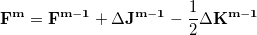 |
(4.94) |
where  is the SCF cycle, and
  J
J and K are computed using the difference density
 |
(4.95) |
Using Schwartz integrals and elements of the difference density, Q-Chem is able to determine at each iteration which ERIs are required, and if necessary, recalculated. As the SCF nears convergence,  becomes sparse and the number of ERIs that need to be recalculated declines dramatically, saving the user large amounts of computational time.
Incremental Fock matrix builds and variable thresholds are only used when the SCF is carried out using the direct SCF algorithm and are clearly complementary algorithms. These options are controlled by the following input parameters, which are only used with direct SCF calculations.
INCFOCK
Iteration number after which the incremental Fock matrix algorithm is initiated
TYPE:
INTEGER
DEFAULT:
1
Start INCFOCK after iteration number 1
OPTIONS:
User-defined (0 switches INCFOCK off)
RECOMMENDATION:
May be necessary to allow several iterations before switching on INCFOCK.
VARTHRESH
Controls the temporary integral cut-off threshold.

TYPE:
INTEGER
DEFAULT:
0
Turns VARTHRESH off
OPTIONS:
User-defined threshold
RECOMMENDATION:
3 has been found to be a practical level, and can slightly speed up SCF evaluation.
4.8.5 Incremental DFT
Incremental DFT (IncDFT) uses the difference density and functional values to improve the performance of the DFT quadrature procedure by providing a better screening of negligible values. Using this option will yield improved efficiency at each successive iteration due to more effective screening.
INCDFT
Toggles the use of the IncDFT procedure for DFT energy calculations.
TYPE:
LOGICAL
DEFAULT:
TRUE
OPTIONS:
FALSE
Do not use IncDFT
TRUE
Use IncDFT
RECOMMENDATION:
Turning this option on can lead to faster SCF calculations, particularly towards the end of the SCF. Please note that for some systems use of this option may lead to convergence problems.
INCDFT_DENDIFF_THRESH
Sets the threshold for screening density matrix values in the IncDFT procedure.
TYPE:
INTEGER
DEFAULT:
SCF_CONVERGENCE + 3
OPTIONS:
Corresponding to a threshold of
.
RECOMMENDATION:
If the default value causes convergence problems, set this value higher to tighten the threshold.
INCDFT_GRIDDIFF_THRESH
Sets the threshold for screening functional values in the IncDFT procedure
TYPE:
INTEGER
DEFAULT:
SCF_CONVERGENCE + 3
OPTIONS:
Corresponding to a threshold of
RECOMMENDATION:
If the default value causes convergence problems, set this value higher to tighten the threshold.
INCDFT_DENDIFF_VARTHRESH
Sets the lower bound for the variable threshold for screening density matrix values in the IncDFT procedure. The threshold will begin at this value and then vary depending on the error in the current SCF iteration until the value specified by INCDFT_DENDIFF_THRESH is reached. This means this value must be set lower than INCDFT_DENDIFF_THRESH.
TYPE:
INTEGER
DEFAULT:
0
Variable threshold is not used.
OPTIONS:
Corresponding to a threshold of
RECOMMENDATION:
If the default value causes convergence problems, set this value higher to tighten accuracy. If this fails, set to 0 and use a static threshold.
INCDFT_GRIDDIFF_VARTHRESH
Sets the lower bound for the variable threshold for screening the functional values in the IncDFT procedure. The threshold will begin at this value and then vary depending on the error in the current SCF iteration until the value specified by INCDFT_GRIDDIFF_THRESH is reached. This means that this value must be set lower than INCDFT_GRIDDIFF_THRESH.
TYPE:
INTEGER
DEFAULT:
0
Variable threshold is not used.
OPTIONS:
Corresponding to a threshold of
RECOMMENDATION:
If the default value causes convergence problems, set this value higher to tighten accuracy. If this fails, set to 0 and use a static threshold.
4.8.6 Fourier Transform Coulomb Method
The Coulomb part of the DFT calculations using ordinary Gaussian representations can be sped up dramatically using plane waves as a secondary basis set by replacing the most costly analytical electron repulsion integrals with numerical integration techniques. The main advantages to keeping the Gaussians as the primary basis set is that the diagonalization step is much faster than using plane waves as the primary basis set, and all electron calculations can be performed analytically.
The Fourier Transform Coulomb (FTC) technique [267, 268] is precise and tunable and all results are practically identical with the traditional analytical integral calculations. The FTC technique is at least 2–3 orders of magnitude more accurate then other popular plane wave based methods using the same energy cutoff. It is also at least 2–3 orders of magnitude more accurate than the density fitting (resolution-of-identity) technique. Recently, an efficient way to implement the forces of the Coulomb energy was introduced [269], and a new technique to localize filtered core functions. Both of these features have been implemented within Q-Chem and contribute to the efficiency of the method.
The FTC method achieves these spectacular results by replacing the analytical integral calculations, whose computational costs scales as  (where
  is the number of basis function) with procedures that scale as only
  . The asymptotic scaling of computational costs with system size is linear versus the analytical integral evaluation which is quadratic. Research at Q-Chem Inc. has yielded a new, general, and very efficient implementation of the FTC method which work in tandem with the J-engine and the CFMM (Continuous Fast Multipole Method) techniques [270].
In the current implementation the speed-ups arising from the FTC technique are moderate when small or medium Pople basis sets are used. The reason is that the J-matrix engine and CFMM techniques provide an already highly efficient solution to the Coulomb problem. However, increasing the number of polarization functions and, particularly, the number of diffuse functions allows the FTC to come into its own and gives the most significant improvements. For instance, using the 6-311G+(df,pd) basis set for a medium-to-large size molecule is more affordable today then before. We found also significant speed ups when non–Pople basis sets are used such as cc-pvTZ. The FTC energy and gradients calculations are implemented to use up to  -type basis functions.
FTC
Controls the overall use of the FTC.
TYPE:
INTEGER
DEFAULT:
0
OPTIONS:
0
Do not use FTC in the Coulomb part
1
Use FTC in the Coulomb part
RECOMMENDATION:
Use FTC when bigger and/or diffuse basis sets are used.
FTC_SMALLMOL
Controls whether or not the operator is evaluated on a large grid and stored in memory to speed up the calculation.
TYPE:
INTEGER
DEFAULT:
1
OPTIONS:
1
Use a big pre-calculated array to speed up the FTC calculations
0
Use this option to save some memory
RECOMMENDATION:
Use the default if possible and use 0 (or buy some more memory) when needed.
FTC_CLASS_THRESH_ORDER
Together with FTC_CLASS_THRESH_MULT, determines the cutoff threshold for included a shell-pair in the
class, i.e., the class that is expanded in terms of plane waves.
TYPE:
INTEGER
DEFAULT:
5
Logarithmic part of the FTC classification threshold. Corresponds to

OPTIONS:
User specified
RECOMMENDATION:
Use the default.
FTC_CLASS_THRESH_MULT
Together with FTC_CLASS_THRESH_ORDER, determines the cutoff threshold for included a shell-pair in the
TYPE:
INTEGER
DEFAULT:
5
Multiplicative part of the FTC classification threshold. Together with
the default value of the FTC_CLASS_THRESH_ORDER this leads to
the
threshold value.
OPTIONS:
User specified.
RECOMMENDATION:
Use the default. If diffuse basis sets are used and the molecule is relatively big then tighter FTC classification threshold has to be used. According to our experiments using Pople-type diffuse basis sets, the default
threshold value for alanine10 and
value for alanine15 has to be used.
4.8.7 Multi-resolution Exchange-Correlation (MRXC) Method
MRXC (multi-resolution exchange-correlation) [271, 272, 273] is a new method developed by the Q-Chem development team for the accelerating the computation of exchange-correlation (XC) energy and matrix originated from the XC functional. As explained in 4.8.6, the XC functional is so complicated that the integration of it is usually done on a numerical quadrature. There are two basic types of quadrature. One is the atom-centered grid (ACG), a superposition of atomic quadrature described in 4.8.6. The ACG has high density of points near the nucleus to handle the compact core density and low density of points in the valence and non-bonding region where the electron density is smooth. The other type is even-spaced cubic grid (ESCG), which is typically used together with pseudopotentials and plane-wave basis functions where only the valence and non-bonded electron density is assumed smooth. In quantum chemistry, an ACG is more often used as it can handle accurately all-electron calculations of molecules. MRXC combines those two integration schemes seamlessly to achieve an optimal computational efficiency by placing the calculation of the smooth part of the density and XC matrix onto the ESCG. The computation associated with the smooth fraction of the electron density is the major bottleneck of the XC part of a DFT calculation and can be done at a much faster rate on the ESCG due to its low resolution. Fast Fourier transform and B-spline interpolation are employed for the accurate transformation between the two types of grids such that the final results remain the same as they would be on the ACG alone. Yet, a speed-up of several times for the calculations of electron-density and XC matrix is achieved. The smooth part of the calculation with MRXC can also be combined with FTC (see section 4.8.6) to achieve further gain of efficiency.
MRXC
Controls the use of MRXC.
TYPE:
INTEGER
DEFAULT:
0
OPTIONS:
0
Do not use MRXC
1
Use MRXC in the evaluation of the XC part
RECOMMENDATION:
MRXC is very efficient for medium and large molecules, especially when medium and large basis sets are used.
The following two keywords control the smoothness precision. The default value is carefully selected to maintain high accuracy.
MRXC_CLASS_THRESH_MULT
Controls the of smoothness precision
TYPE:
INTEGER
DEFAULT:
1
OPTIONS:

An integer
RECOMMENDATION:
A prefactor in the threshold for MRXC error control:

MRXC_CLASS_THRESH_ORDER
Controls the of smoothness precision
TYPE:
INTEGER
DEFAULT:
6
OPTIONS:

An integer
RECOMMENDATION:
The exponent in the threshold of the MRXC error control:
The next keyword controls the order of the B-spline interpolation:
LOCAL_INTERP_ORDER
Controls the order of the B-spline
TYPE:
INTEGER
DEFAULT:
6
OPTIONS:
An integer
RECOMMENDATION:
The default value is sufficiently accurate
4.8.8 Resolution of the Identity Fock Matrix Methods
Evaluation of the Fock matrix (both Coulomb, J, and exchange, K, pieces) can be sped up by an approximation known as the resolution-of-the-identity approximation (RI-JK). Essentially, the full complexity in common basis sets required to describe chemical bonding is not necessary to describe the mean-field Coulomb and exchange interactions between electrons. That is,  in the left side of
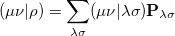 |
(4.96) |
is much less complicated than an individual  function pair. The same principle applies to the FTC method in subsection 4.8.6, in which case the slowly varying piece of the electron density is replaced with a plane-wave expansion.
With the RI-JK approximation, the Coulomb interactions of the function pair 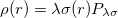 are fit by a smaller set of atom-centered basis functions. In terms of J:
 |
(4.97) |
The coefficients  must be determined to accurately represent the potential. This is done by performing a least-squared minimization of the difference between
  and
and  , with differences measured by the Coulomb metric. This requires a matrix inversion over the space of auxiliary basis functions, which may be done rapidly by Cholesky decomposition.
The RI method applied to the Fock matrix may be further enhanced by performing local fitting of a density or function pair element. This is the basis of the atomic-RI method (ARI), which has been developed for both Coulomb (J) matrix [274] and exchange (K) matrix evaluation [275]. In ARI, only nearby auxiliary functions  are employed to fit the target function. This reduces the asymptotic scaling of the matrix-inversion step as well as that of many intermediate steps in the digestion of RI integrals. Briefly, atom-centered auxiliary functions on nearby atoms are only used if they are within the “outer” radius (
 ) of the fitting region. Between and the “inner” radius (
 ), the amplitude of interacting auxiliary functions is smoothed by a function that goes from zero to one and has continuous derivatives. To optimize efficiency, the van der Waals radius of the atom is included in the cutoff so that smaller atoms are dropped from the fitting radius sooner. The values of and are specified as REM variables as described below.
RI_J
Toggles the use of the RI algorithm to compute J.
TYPE:
LOGICAL
DEFAULT:
FALSE
RI will not be used to compute J.
OPTIONS:
TRUE
Turn on RI for J.
RECOMMENDATION:
For large (especially 1D and 2D) molecules the approximation may yield significant improvements in Fock evaluation time when used with ARI.
RI_K
Toggles the use of the RI algorithm to compute K.
TYPE:
LOGICAL
DEFAULT:
FALSE
RI will not be used to compute K.
OPTIONS:
TRUE
Turn on RI for K.
RECOMMENDATION:
For large (especially 1D and 2D) molecules the approximation may yield significant improvements in Fock evaluation time when used with ARI.
ARI
Toggles the use of the atomic resolution-of-the-identity (ARI) approximation.
TYPE:
LOGICAL
DEFAULT:
FALSE
ARI will not be used by default for an RI-JK calculation.
OPTIONS:
TRUE
Turn on ARI.
RECOMMENDATION:
For large (especially 1D and 2D) molecules the approximation may yield significant improvements in Fock evaluation time.
ARI_R0
Determines the value of the inner fitting radius (in ngstroms)
TYPE:
INTEGER
DEFAULT:
4
A value of 4 will be added to the atomic van der Waals radius.
OPTIONS:
User defined radius.
RECOMMENDATION:
For some systems the default value may be too small and the calculation will become unstable.
ARI_R1
Determines the value of the outer fitting radius (in ngstroms)
TYPE:
INTEGER
DEFAULT:
5
A value of 5 will be added to the atomic van der Waals radius.
OPTIONS:
User defined radius.
RECOMMENDATION:
For some systems the default value may be too small and the calculation will become unstable. This value also determines, in part, the smoothness of the potential energy surface.
4.8.9 PARI-K Fast Exchange Algorithm
PARI-K[276] is an algorithm that significantly accelerates the construction of the exchange matrix in Hartree-Fock and hybrid density functional theory calculations with large basis sets. The speedup is made possible by fitting products of atomic orbitals using only auxiliary basis functions found on their respective atoms. The PARI-K implementation in Q-Chem is an efficient MO-basis formulation similar to the AO-basis formulation of Merlot et al. [277]. PARI-K is highly recommended for calculations using basis sets of size augmented triple-zeta or larger, and should be used in conjunction with the standard RI-J algorithm [278] for constructing the Coulomb matrix. The exchange fitting basis sets of Weigend (cc-pVTZ-JK and cc-pVQZ-JK) [278] are recommended for use in conjunction with PARI-K. The errors associated with the PARI-K approximation appear to be only slightly worse than standard RI-HF [277].
PARI_K
Controls the use of the PARI-K approximation in the construction of the exchange matrix
TYPE:
LOGICAL
DEFAULT:
FALSE
Do not use PARI-K.
OPTIONS:
TRUE
Use PARI-K.
RECOMMENDATION:
Use for basis sets aug-cc-pVTZ and larger.
4.8.10 CASE Approximation
The Coulomb Attenuated Schrödinger Equation (CASE) [279] approximation follows from the KWIK [280] algorithm in which the Coulomb operator is separated into two pieces using the error function, Eq. (). Whereas in Section 4.4.6 this partition of the Coulomb operator was used to incorporate long-range Hartree-Fock exchange into DFT, within the CASE approximation it is used to attenuate all occurrences of the Coulomb operator in Eq. (4.2), by neglecting the long-range portion of the identity in Eq. (). The parameter  in Eq. () is used to tune the level of attenuation. Although the total energies from Coulomb attenuated calculations are significantly different from non-attenuated energies, it is found that relative energies, correlation energies and, in particular, wave functions, are not, provided a reasonable value of is chosen.
By virtue of the exponential decay of the attenuated operator, ERIs can be neglected on a proximity basis yielding a rigorous  algorithm for single point energies. CASE may also be applied in geometry optimizations and frequency calculations.
OMEGA
Controls the degree of attenuation of the Coulomb operator.
TYPE:
INTEGER
DEFAULT:
No default
OPTIONS:
Corresponding to
, in units of bohr

RECOMMENDATION:
None
INTEGRAL_2E_OPR
Determines the two-electron operator.
TYPE:
INTEGER
DEFAULT:
-2
Coulomb Operator.
OPTIONS:
-1
Apply the CASE approximation.
-2
Coulomb Operator.
RECOMMENDATION:
Use the default unless the CASE operator is desired.
4.8.11 occ-RI-K Exchange Algorithm
The occupied orbital RI-K (occ-RI-K) [281] is a new scheme for building the exchange matrix (K) partially in the MO basis using the RI approximation. occ-RI-K typically matches current alternatives in terms of both the accuracy (energetics identical to standard RI-K) and convergence (essentially unchanged relative to conventional methods). On the other hand, this algorithm exhibits significant speedups over conventional integral evaluation (14x) and standard RI-K (3.3x) for a test system, a graphene fragment (C H
H ) using cc-pVQZ basis set (4400 basis functions), whereas the speedup increases with the size of the AO basis set. Thus occ-RI-K helps to make larger basis set hybrid DFT calculations more feasible, which is quite desirable for achieving improved accuracy in DFT calculations with modern functionals.
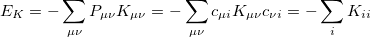
The idea of the occ-RI-K formalism comes from a simple observation that the exchange energy  and its gradient can be evaluated from the diagonal elements of the exchange matrix in the occupied-occupied block
  , and occupied-virtual block
  , respectively, rather than the full matrix in the AO representation,
  . Mathematically,
 |
(4.98) |
and
 |
(4.99) |
where is a skew-symmetric matrix used to parameterize the unitary transformation  , which represents the variations of the MO coefficients as follows:
 |
(4.100) |
From Eq. 4.98 and 4.99 it is evident that the exchange energy and gradient need just  rather than .
In regular RI-K [278] one has to compute two quartic terms, whereas there are three quartic terms for the occ-RI-K algorithm. The speedup of the latter with respect to former can be explained from the following ratio of operations (refer to [281] for detail),
 |
(4.101) |
With a conservative approximation of  , the speedup is
  . The occ-RI-K algorithm also involves some cubic steps which should be negligible in the very large molecule limit. Tests in the Ref. Manzer:2015b suggest that occ-RI-K for small systems with large basis will gain less speed than a large system with small basis, because the cubic terms will be more dominant for the former than the latter case.
In the course of SCF iteration, the occ-RI-K method does not require us to construct the exact Fock matrix explicitly. Rather,  contributes to the Fock matrix in the mixed MO and AO representations (
 ) and yields orbital gradient and DIIS error vectors for converging SCF. On the other hand, since occ-RI-K does not provide exactly the same unoccupied eigenvalues, the diagonalization updates can differ from the conventional SCF procedure. In Ref. Manzer:2015b, occ-RI-K was found to require, on average, the same number of SCF iterations to converge and to yield accurate energies.
OCC_RI_K
Controls the use of the occ-RI-K approximation for constructing the exchange matrix
TYPE:
LOGICAL
DEFAULT:
False
Do not use occ-RI-K.
OPTIONS:
True
Use occ-RI-K.
RECOMMENDATION:
Larger the system, better the performance
4.8.11.1 occ-RI-K for exchange energy gradient evaluation
A very attractive feature of occ-RI-K framework is that one can compute the exchange energy gradient with respect to nuclear coordinates with the same leading quartic-scaling operations as the energy calculation.
The occ-RI-K formulation yields the following formula for the gradient of exchange energy in global Coulomb-metric RI:
 |
 |
 |
|||
 |
|
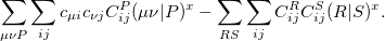 |
(4.102) |
The superscript  represents the derivative with respect to a nuclear coordinate. Note that the derivatives of the MO coefficients
  are not included here, because they are already included in the total energy derivative calculation by Q-Chem via the derivative of the overlap matrix.
In Eq. 4.102, the construction of the density fitting coefficients ( ) has the worst scaling of
  because it involves MO to AO back transformations:
 |
(4.103) |
where the operation cost is ![$ o^2NX + o[\mathrm{NB2}]X $](images/img-0469.png) .
.
RI_K_GRAD
Turn on the nuclear gradient calculations
TYPE:
LOGICAL
DEFAULT:
FALSE
Do not invoke occ-RI-K based gradient
OPTIONS:
TRUE
Use occ-RI-K based gradient
RECOMMENDATION:
Use "RI_J false"
4.8.12 Examples
Example 4.59 Q-Chem input for a large single point energy calculation. The CFMM is switched on automatically when LinK is requested.
$comment
   HF/3-21G single point calculation on a large molecule
   read in the molecular coordinates from file
$end

$molecule
   read dna.inp
$end

$rem
   METHOD     HF      Hartree-Fock
   BASIS      3-21G   Basis set
   LIN_K      TRUE    Calculate K using LinK
$end
Example 4.60 Q-Chem input for a large single point energy calculation. This would be appropriate for a medium-sized molecule, but for truly large calculations, the CFMM and LinK algorithms are far more efficient.
$comment
   HF/3-21G single point calculation on a large molecule
   read in the molecular coordinates from file
$end

$molecule
   read dna.inp
$end

$rem
   METHOD      HF      Hartree-Fock
   BASIS       3-21G   Basis set
   INCFOCK     5       Incremental Fock after 5 cycles
   VARTHRESH   3       1.0d-03 variable threshold
$end
Example 4.61 Q-Chem input for a energy and gradient calculations with occ-RI-K method.
$molecule
   read  C30H62.inp
$end

$rem
   JOBTYPE         force
   EXCHANGE        HF
   BASIS           cc-pVDZ
   AUX_BASIS       cc-pVTZ-JK
   OCC_RI_K        1
   RI_K_GRAD       1
   INCFOCK         0
   PURECART        1111
$end