10.17 Electronic Couplings for Electron Transfer and Energy Transfer
10.17.1 Eigenstate-Based Methods
For electron transfer (ET) and excitation energy transfer (EET) processes, the electronic coupling is one of the important parameters that determine their reaction rates. For ET, Q-Chem provides the coupling values calculated with the generalized Mulliken-Hush (GMH) [700], fragment-charge difference (FCD) [701], Boys localization [702], and Edmiston-Ruedenbeg localization [703] schemes. For EET, options include fragment-excitation difference (FED) [704], fragment-spin difference (FSD) [705], occupied-virtual separated Boys localization [706] or Edmiston-Ruedenberg localization [703]. In all these schemes, a vertical excitation such as CIS, RPA or TDDFT is required, and the GMH, FCD, FED, FSD, Boys or ER coupling values are calculated based on the excited state results.
10.17.1.1 Two-state approximation
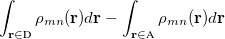
Under the two-state approximation, the diabatic reactant and product states are assumed to be a linear combination of the eigenstates. For ET, the choice of such linear combination is determined by a zero transition dipoles (GMH) or maximum charge differences (FCD). In the latter, a  donor–acceptor charge difference matrix,
  , is defined, with elements
 |
 |
 |
|||
 |
|
 |
(10.68) |
where  is the matrix element of the density operator between states
  and
and  .
.
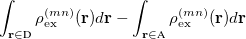
For EET, a maximum excitation difference is assumed in the FED, in which a excitation difference matrix is similarly defined with elements
 |
 |
||||
|
|
 |
(10.69) |
where  is the sum of attachment and detachment densities for transition
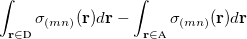
  , as they correspond to the electron and hole densities in an excitation. In the FSD, a maximum spin difference is used and the corresponding spin difference matrix is defined with its elements as,
 |
|
 |
|||
|
|
 |
(10.70) |
where  is the spin density, difference between
  -spin and
  -spin densities, for transition from .
Since Q-Chem uses a Mulliken population analysis for the integrations in Eqs. (10.68), (10.69), and (10.70), the matrices ,  and
and  are not symmetric. To obtain a pair of orthogonal states as the diabatic reactant and product states, , and are symmetrized in Q-Chem. Specifically,
 |
 |
 |
(10.71) | ||
 |
|
 |
(10.72) | ||
 |
|
 |
(10.73) |
The final coupling values are obtained as listed below:
For GMH,
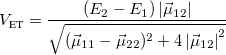
(10.74) For FCD,
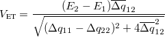
(10.75) For FED,
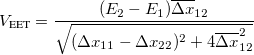
(10.76) For FSD,
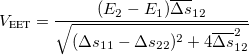
(10.77)
Q-Chem provides the option to control FED, FSD, FCD and GMH calculations after a single-excitation calculation, such as CIS, RPA, TDDFT/TDA and TDDFT. To obtain ET coupling values using GMH (FCD) scheme, one should set $rem variables STS_GMH (STS_FCD) to be TRUE. Similarly, a FED (FSD) calculation is turned on by setting the $rem variable STS_FED (STS_FSD) to be TRUE. In FCD, FED and FSD calculations, the donor and acceptor fragments are defined via the $rem variables STS_DONOR and STS_ACCEPTOR. It is necessary to arrange the atomic order in the $molecule section such that the atoms in the donor (acceptor) fragment is in one consecutive block. The ordering numbers of beginning and ending atoms for the donor and acceptor blocks are included in $rem variables STS_DONOR and STS_ACCEPTOR.
The couplings will be calculated between all choices of excited states with the same spin. In FSD, FCD and GMH calculations, the coupling value between the excited and reference (ground) states will be included, but in FED, the ground state is not included in the analysis. It is important to select excited states properly, according to the distribution of charge or excitation, among other characteristics, such that the coupling obtained can properly describe the electronic coupling of the corresponding process in the two-state approximation.
STS_GMH
Control the calculation of GMH for ET couplings.
TYPE:
LOGICAL
DEFAULT:
FALSE
OPTIONS:
FALSE
Do not perform a GMH calculation.
TRUE
Include a GMH calculation.
RECOMMENDATION:
When set to true computes Mulliken-Hush electronic couplings. It yields the generalized Mulliken-Hush couplings as well as the transition dipole moments for each pair of excited states and for each excited state with the ground state.
STS_FCD
Control the calculation of FCD for ET couplings.
TYPE:
LOGICAL
DEFAULT:
FALSE
OPTIONS:
FALSE
Do not perform an FCD calculation.
TRUE
Include an FCD calculation.
RECOMMENDATION:
None
STS_FED
Control the calculation of FED for EET couplings.
TYPE:
LOGICAL
DEFAULT:
FALSE
OPTIONS:
FALSE
Do not perform a FED calculation.
TRUE
Include a FED calculation.
RECOMMENDATION:
None
STS_FSD
Control the calculation of FSD for EET couplings.
TYPE:
LOGICAL
DEFAULT:
FALSE
OPTIONS:
FALSE
Do not perform a FSD calculation.
TRUE
Include a FSD calculation.
RECOMMENDATION:
For RCIS triplets, FSD and FED are equivalent. FSD will be automatically switched off and perform a FED calculation.
STS_DONOR
Define the donor fragment.
TYPE:
STRING
DEFAULT:
0
No donor fragment is defined.
OPTIONS:
-

Donor fragment is in the
RECOMMENDATION:
Note no space between the hyphen and the numbers
STS_ACCEPTOR
Define the acceptor molecular fragment.
TYPE:
STRING
DEFAULT:
0
No acceptor fragment is defined.
OPTIONS:
Acceptor fragment is in the
RECOMMENDATION:
Note no space between the hyphen and the numbers
STS_MOM
Control calculation of the transition moments between excited states in the CIS and TDDFT calculations (including SF variants).
TYPE:
LOGICAL
DEFAULT:
FALSE
OPTIONS:
FALSE
Do not calculate state-to-state transition moments.
TRUE
Do calculate state-to-state transition moments.
RECOMMENDATION:
When set to true requests the state-to-state dipole transition moments for all pairs of excited states and for each excited state with the ground state.
Example 10.258 A GMH & FCD calculation to analyze electron-transfer couplings in an ethylene and a methaniminium cation.
$molecule
   1  1
   C     0.679952    0.000000    0.000000
   N    -0.600337    0.000000    0.000000
   H     1.210416    0.940723    0.000000
   H     1.210416   -0.940723    0.000000
   H    -1.131897   -0.866630    0.000000
   H    -1.131897    0.866630    0.000000
   C    -5.600337    0.000000    0.000000
   C    -6.937337    0.000000    0.000000
   H    -5.034682    0.927055    0.000000
   H    -5.034682   -0.927055    0.000000
   H    -7.502992   -0.927055    0.000000
   H    -7.502992    0.927055    0.000000
$end

$rem
   METHOD        CIS
   BASIS         6-31+G
   CIS_N_ROOTS   20
   CIS_SINGLETS  true
   CIS_TRIPLETS  false
   STS_GMH       true !turns on the GMH calculation
   STS_FCD       true !turns on the FCD calculation
   STS_DONOR     1-6  !define the donor fragment as atoms 1-6 for FCD calc.
   STS_ACCEPTOR  7-12 !define the acceptor fragment as atoms 7-12 for FCD calc.
   MEM_STATIC    200  !increase static memory for a CIS job with larger basis set
$end
Example 10.259 An FED calculation to analyze excitation-energy transfer couplings in a pair of stacked ethylenes.
$molecule
   0  1
   C     0.670518    0.000000    0.000000
   H     1.241372    0.927754    0.000000
   H     1.241372   -0.927754    0.000000
   C    -0.670518    0.000000    0.000000
   H    -1.241372   -0.927754    0.000000
   H    -1.241372    0.927754    0.000000
   C     0.774635    0.000000    4.500000
   H     1.323105    0.936763    4.500000
   H     1.323105   -0.936763    4.500000
   C    -0.774635    0.000000    4.500000
   H    -1.323105   -0.936763    4.500000
   H    -1.323105    0.936763    4.500000
$end

$rem
   METHOD            CIS
   BASIS             3-21G
   CIS_N_ROOTS       20
   CIS_SINGLETS      true
   CIS_TRIPLETS      false
   STS_FED           true
   STS_DONOR         1-6
   STS_ACCEPTOR      7-12
$end
10.17.1.2 Multi-state treatments
When dealing with multiple charge or electronic excitation centers, diabatic states can be constructed with Boys [702] or Edmiston-Ruedenberg [703] localization. In this case, we construct diabatic states  as linear combinations of adiabatic states
  with a general rotation matrix
  that is
  in size:
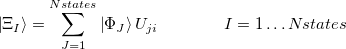 |
(10.78) |
The adiabatic states can be produced with any method, in principle, but the Boys/ER-localized diabatization methods have been implemented thus far only for CIS or TDDFT methods in Q-Chem. In analogy to orbital localization, Boys-localized diabatization corresponds to maximizing the charge separation between diabatic state centers:
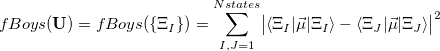 |
(10.79) |
Here,  represents the dipole operator. ER-localized diabatization prescribes maximizing self-interaction energy:
 |
|
 |
(10.80) | ||
 |
|
 |
where the density operator at position  is
is
 |
(10.81) |
Here,  represents the position of the th electron.
These models reflect different assumptions about the interaction of our quantum system with some fictitious external electric field/potential:  if we assume a fictitious field that is linear in space, we arrive at Boys localization;
  if we assume a fictitious potential energy that responds linearly to the charge density of our system, we arrive at ER localization. Note that in the two-state limit, Boys localized diabatization reduces nearly exactly to GMH [702].
As written down in Eq. (10.79), Boys localized diabatization applies only to charge transfer, not to energy transfer. Within the context of CIS or TDDFT calculations, one can easily extend Boys localized diabatization [706] by separately localizing the occupied and virtual components of ,  and
and  :
:
 |
|
 |
(10.82) | ||
|
|
 |
where
 |
(10.83) |
and the occupied/virtual components are defined by
 |
|
 |
(10.84) | ||
|
|
 |
Note that when we maximize the Boys OV function, we are simply performing Boys-localized diabatization separately on the electron attachment and detachment densities.
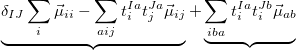
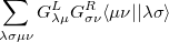
Finally, for energy transfer, it can be helpful to understand the origin of the diabatic couplings. To that end, we now provide the ability to decompose the diabatic coupling between diabatic states into Coulomb (J), Exchange (K) and one-electron (O) components [707]:
 |
|
 |
|||
|
|
 |
(10.85) |
BOYS_CIS_NUMSTATE
Define how many states to mix with Boys localized diabatization. These states must be specified in the $localized_diabatization section.
TYPE:
INTEGER
DEFAULT:
0
Do not perform Boys localized diabatization.
OPTIONS:
2 to N where N is the number of CIS states requested (CIS_N_ROOTS)
RECOMMENDATION:
It is usually not wise to mix adiabatic states that are separated by more than a few eV or a typical reorganization energy in solvent.
ER_CIS_NUMSTATE
Define how many states to mix with ER localized diabatization. These states must be specified in the $localized_diabatization section.
TYPE:
INTEGER
DEFAULT:
0
Do not perform ER localized diabatization.
OPTIONS:
2 to N where N is the number of CIS states requested (CIS_N_ROOTS)
RECOMMENDATION:
It is usually not wise to mix adiabatic states that are separated by more than a few eV or a typical reorganization energy in solvent.
LOC_CIS_OV_SEPARATE
Decide whether or not to localized the “occupied” and “virtual” components of the localized diabatization function, i.e., whether to localize the electron attachments and detachments separately.
TYPE:
LOGICAL
DEFAULT:
FALSE
Do not separately localize electron attachments and detachments.
OPTIONS:
TRUE
RECOMMENDATION:
If one wants to use Boys localized diabatization for energy transfer (as opposed to electron transfer) , this is a necessary option. ER is more rigorous technique, and does not require this OV feature, but will be somewhat slower.
CIS_DIABATH_DECOMPOSE
Decide whether or not to decompose the diabatic coupling into Coulomb, exchange, and one-electron terms.
TYPE:
LOGICAL
DEFAULT:
FALSE
Do not decompose the diabatic coupling.
OPTIONS:
TRUE
RECOMMENDATION:
These decompositions are most meaningful for electronic excitation transfer processes. Currently, available only for CIS, not for TDDFT diabatic states.
Example 10.260 A calculation using ER localized diabatization to construct the diabatic Hamiltonian and couplings between a square of singly-excited Helium atoms.
$molecule
   0 1
   he   0  -1.0    1.0
   he   0  -1.0   -1.0
   he   0   1.0   -1.0
   he   0   1.0    1.0
$end

$rem
   method                 cis
   cis_n_roots            4
   cis_singles            false
   cis_triplets           true
   basis                  6-31g**
   scf_convergence        8
   symmetry               false
   rpa                    false
   sym_ignore             true
   sym_ignore             true
   loc_cis_ov_separate    false  ! NOT localizing attachments/detachments separately.
   er_cis_numstate        4      ! using ER to mix 4 adiabatic states.
   cis_diabatH_decompose  true   ! decompose diabatic couplings into
                                 ! Coulomb, exchange, and one-electron components.
$end

$localized_diabatization
   On the next line, list which excited adiabatic states we want to mix.
   1 2 3 4
$end
10.17.2 Diabatic-State-Based Methods
10.17.2.1 Electronic coupling in charge transfer
A charge transfer involves a change in the electron numbers in a pair of molecular fragments. As an example, we will use the following reaction when necessary, and a generalization to other cases is straightforward:
 |
(10.86) |
where an extra electron is localized to the donor (D) initially, and it becomes localized to the acceptor (A) in the final state. The two-state secular equation for the initial and final electronic states can be written as
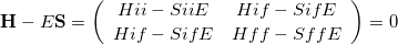 |
(10.87) |
This is very close to an eigenvalue problem except for the non-orthogonality between the initial and final states. A standard eigenvalue form for Eq. (10.87) can be obtained by using the Löwdin transformation:
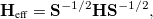 |
(10.88) |
where the off-diagonal element of the effective Hamiltonian matrix represents the electronic coupling for the reaction, and it is defined by
 |
(10.89) |
In a general case where the initial and final states are not normalized, the electronic coupling is written as
 |
(10.90) |
Thus, in principle,  can be obtained when the matrix elements for the Hamiltonian
  and the overlap matrix
  are calculated.
The direct coupling (DC) scheme calculates the electronic coupling values via Eq. (10.90), and it is widely used to calculate the electron transfer coupling [708, 709, 710, 711]. In the DC scheme, the coupling matrix element is calculated directly using charge-localized determinants (the “diabatic states” in electron transfer literature). In electron transfer systems, it has been shown that such charge-localized states can be approximated by symmetry-broken unrestricted Hartree-Fock (UHF) solutions [708, 709, 712]. The adiabatic eigenstates are assumed to be the symmetric and anti-symmetric linear combinations of the two symmetry-broken UHF solutions in a DC calculation. Therefore, DC couplings can be viewed as a result of two-configuration solutions that may recover the non-dynamical correlation.
The core of the DC method is based on the corresponding orbital transformation [713] and a calculation for Slater’s determinants in  and
and  [710, 711].
10.17.2.2 Corresponding orbital transformation
Let  and
and  be two single Slater-determinant wave functions for the initial and final states, and
  and
and  be the spin-orbital sets, respectively:
 |
|
 |
(10.91) | ||
 |
|
 |
(10.92) |
Since the two sets of spin-orbitals are not orthogonal, the overlap matrix  can be defined as:
 |
(10.93) |
We note that is not Hermitian in general since the molecular orbitals of the initial and final states are separately determined. To calculate the matrix elements  and
and  , two sets of new orthogonal spin-orbitals can be used by the corresponding orbital transformation [713]. In this approach, each set of spin-orbitals and are linearly transformed,
 |
|
 |
(10.94) | ||
 |
|
 |
(10.95) |
where  and
and  are the left-singular and right-singular matrices, respectively, in the singular value decomposition (SVD) of :
 |
(10.96) |
The overlap matrix in the new basis is now diagonal
 |
(10.97) |
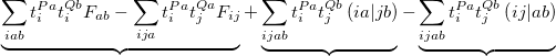
10.17.2.3 Generalized density matrix
The Hamiltonian for electrons in molecules are a sum of one-electron and two-electron operators. In the following, we derive the expressions for the one-electron operator  and two-electron operator
  ,
,
 |
|
 |
(10.98) | ||
 |
|
 |
(10.99) |
where  and
and  , for the molecular Hamiltonian, are
 |
(10.100) |
and
 |
(10.101) |
The evaluation of matrix elements can now proceed:
 |
(10.102) |
 |
(10.103) |
 |
(10.104) |
 |
(10.105) |
In an atomic orbital basis set,  , we can expand the molecular spin orbitals and ,
 |
(10.106) | ||
 |
(10.107) |
The one-electron terms, Eq. (10.102), can be expressed as
 |
|
 |
|||
 |
|
 |
(10.108) |
where  and define a generalized density matrix,
  :
:
 |
|
 |
(10.109) |
Similarly, the two-electron terms, Eq. (10.104), are
 |
|
 |
|||
 |
|
 |
(10.110) |
where  and
and  are generalized density matrices as defined in Eq. (10.109) except
  in is replaced by
  .
.
The - and -spin orbitals are treated explicitly. In terms of the spatial orbitals, the one- and two-electron contributions can be reduced to
|
|
 |
(10.111) | ||
 |
|
 |
|||
|
|
 |
(10.112) |
The resulting one- and two-electron contributions, Eqs. (10.111) and (10.112) can be easily computed in terms of generalized density matrices using standard one- and two-electron integral routines in Q-Chem.
10.17.2.4 Direct coupling method for electronic coupling
It is important to obtain proper charge-localized initial and final states for the DC scheme, and this step determines the quality of the coupling values. Q-Chem provides two approaches to construct charge-localized states:
The “1+1” approach
Since the system consists of donor and acceptor molecules or fragments, with a charge being localized either donor or acceptor, it is intuitive to combine wave functions of individual donor and acceptor fragments to form a charge-localized wave function. We call this approach “1+1” since the zeroth order wave functions are composed of the HF wave functions of the two fragments.For example, for the case shown in Example (10.86), we can use Q-Chem to calculate two HF wave functions: those of anionic donor and of neutral acceptor and they jointly form the initial state. For the final state, wave functions of neutral donor and anionic acceptor are used. Then the coupling value is calculated via Eq. (10.90).
Example 10.261 To calculate the electron-transfer coupling for a pair of stacked-ethylene with “1+1” charge-localized states
$molecule
  -1  2
--
  -1  2,  0  1
   C    0.662489    0.000000    0.000000
   H    1.227637    0.917083    0.000000
   H    1.227637   -0.917083    0.000000
   C   -0.662489    0.000000    0.000000
   H   -1.227637   -0.917083    0.000000
   H   -1.227637    0.917083    0.000000
--
   0  1, -1  2
   C    0.720595    0.000000    4.5
   H    1.288664    0.921368    4.5
   H    1.288664   -0.921368    4.5
   C   -0.720595    0.000000    4.5
   H   -1.288664   -0.921368    4.5
   H   -1.288664    0.921368    4.5
$end

$rem
   JOBTYPE           SP
   METHOD            HF
   BASIS             6-31G(d)
   SCF_PRINT_FRGM    FALSE
   SYM_IGNORE        TRUE
   SCF_GUESS         FRAGMO
   STS_DC            TRUE
$end
In the $molecule subsection, the first line is for the charge and multiplicity of the whole system. The following blocks are two inputs for the two molecular fragments (donor and acceptor). In each block the first line consists of the charge and spin multiplicity in the initial state of the corresponding fragment, a comma, then the charge and multiplicity in the final state. Next lines are nuclear species and their positions of the fragment. For example, in the above example, the first block indicates that the electron donor is a doublet ethylene anion initially, and it becomes a singlet neutral species in the final state. The second block is for another ethylene going from a singlet neutral molecule to a doublet anion.
Note that the last three $rem variables in this example, SYM_IGNORE, SCF_GUESS and STS_DC must be set to be the values as in the example in order to perform DC calculation with “1+1” charge-localized states. An additional $rem variable, SCF_PRINT_FRGM is included. When it is TRUE a detailed output for the fragment HF self-consistent field calculation is given.
The “relaxed” approach
In “1+1” approach, the intermolecular interaction is neglected in the initial and final states, and so the final electronic coupling can be underestimated. As a second approach, Q-Chem can use “1+1” wave function as an initial guess to look for the charge-localized wave function by further HF self-consistent field calculation. This approach would ‘relax’ the wave function constructed by “1+1” method and include the intermolecular interaction effects in the initial and final wave functions. However, this method may sometimes fail, leading to either convergence problems or a resulting HF wave function that cannot represent the desired charge-localized states. This is more likely to be a problem when calculations are performed with diffusive basis functions, or when the donor and acceptor molecules are very close to each other.To perform relaxed DC calculation, set STS_DC = RELAX.