A.7 GDIIS

Direct inversion in the iterative subspace (DIIS) was originally developed by Pulay for accelerating SCF convergence [164]. Subsequently, Csaszar and Pulay used a similar scheme for geometry optimization, which they termed GDIIS [727]. The method is somewhat different from the usual quasi-Newton type approach and is included in Optimize as an alternative to the EF algorithm. Tests indicate that its performance is similar to EF, at least for small systems; however there is rarely an advantage in using GDIIS in preference to EF.

In GDIIS, geometries $\ensuremath{\mathbf{x}}_ i$ generated in previous optimization cycles are linearly combined to find the “best” geometry on the current cycle

$\begin{equation} \label{eq:a23} \ensuremath{\mathbf{x}}_ n = \sum \limits _{i=1}^ m c_ i \ensuremath{\mathbf{x}}_ i \end{equation}$

(A.33)

where the problem is to find the best values for the coefficients $c_ i$ .

If we express each geometry, $\ensuremath{\mathbf{x}}_ i$ , by its deviation from the sought-after final geometry, $\ensuremath{\mathbf{x}}_ f$ , i.e., $\ensuremath{\mathbf{x}}_ f = \ensuremath{\mathbf{x}}_ i + \ensuremath{\mathbf{e}}_ i$ , where $\ensuremath{\mathbf{e}}_ i$ is an error vector, then it is obvious that if the conditions

$\begin{equation} \label{eq:a24} \ensuremath{\mathbf{r}} = \sum c_ i \ensuremath{\mathbf{e}}_ i \end{equation}$

(A.34)

and

$\begin{equation} \label{eq:a25} \sum {c_ i} = 1 \end{equation}$

(A.35)

are satisfied, then the relation

$\begin{equation} \sum c_ i \ensuremath{\mathbf{x}}_ i = \ensuremath{\mathbf{x}}_ f \end{equation}$

(A.36)

also holds.

The true error vectors $\ensuremath{\mathbf{e}}_ i$ are, of course, unknown. However, in the case of a nearly quadratic energy function they can be approximated by

$\begin{equation} \ensuremath{\mathbf{e}}_ i = -\ensuremath{\mathbf{H}}^{-1}\ensuremath{\mathbf{g}}_ i \end{equation}$

(A.37)

where $\ensuremath{\mathbf{g}}_ i$ is the gradient vector corresponding to the geometry $\ensuremath{\mathbf{x}}_ i$ and $\ensuremath{\mathbf{H}}$ is an approximation to the Hessian matrix. Minimization of the norm of the residuum vector $\ensuremath{\mathbf{r}}$ , Eq. (A.34), together with the constraint equation, Eq. (A.35), leads to a system of ( $m+l$ ) linear equations

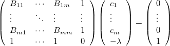$\begin{equation} \label{eq:a28} \left( {{\begin{array}{*{20}c} {B_{11} } \hfill & \cdots \hfill & {B_{1m} } \hfill & 1 \hfill \\ \vdots \hfill & \ddots \hfill & \vdots \hfill & \vdots \hfill \\ {B_{m1} } \hfill & \cdots \hfill & {B_{mm} } \hfill & 1 \hfill \\ 1 \hfill & \cdots \hfill & 1 \hfill & 0 \hfill \\ \end{array} }} \right)\left( {{\begin{array}{*{20}c} {c_1 } \hfill \\ \vdots \hfill \\ {c_ m } \hfill \\ {-\lambda } \hfill \\ \end{array} }} \right)=\left( {{\begin{array}{*{20}c} 0 \hfill \\ \vdots \hfill \\ 0 \hfill \\ 1 \hfill \\ \end{array} }} \right) \end{equation}$

(A.38)

where $B_{ij} = \ensuremath{\langle }\ensuremath{\mathbf{e}}_ i|\ensuremath{\mathbf{e}}_ j\ensuremath{\rangle }$ is the scalar product of the error vectors $\ensuremath{\mathbf{e}}_ i$ and $\ensuremath{\mathbf{e}}_ j$ , and $\lambda$ is a Lagrange multiplier.

The coefficients $c_ i$ determined from Eq. (A.38) are used to calculate an intermediate interpolated geometry

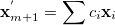$\begin{equation} \ensuremath{\mathbf{x}}_{m+1}^{'} = \sum c_ i \ensuremath{\mathbf{x}}_ i \end{equation}$

(A.39)

and its corresponding interpolated gradient

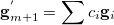$\begin{equation} \ensuremath{\mathbf{g}}_{m+1}^{'} = \sum c_ i \ensuremath{\mathbf{g}}_ i \end{equation}$

(A.40)

A new, independent geometry is generated from the interpolated geometry and gradient according to

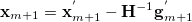$\begin{equation} \ensuremath{\mathbf{x}}_{m+1} = \ensuremath{\mathbf{x}}_{m+1}^{'} - \ensuremath{\mathbf{H}}^{-1} \ensuremath{\mathbf{g}}_{m+1}^{'} \end{equation}$

(A.41)

Note: Convergence is theoretically guaranteed regardless of the quality of the Hessian matrix (as long as it is positive definite), and the original GDIIS algorithm used a static Hessian (i.e., the original starting Hessian, often a simple unit matrix, remained unchanged during the entire optimization). However, updating the Hessian at each cycle generally results in more rapid convergence, and this is the default in Optimize.

Other modifications to the original method include limiting the number of previous geometries used in Eq. (A.33) and, subsequently, by neglecting earlier geometries, and eliminating any geometries more than a certain distance (default: 0.3 a.u.) from the current geometry.