9.4 Minimum-Energy Crossing Points
Conical intersections are the regions of the potential energy surface characterized by degeneracy between two or more electronic states with the same symmetry. For a two-state intersection, the intersection consists of an  -dimensional hypersurface (the seam space) within which the two states are degenerate, where
  is the number of internal coordinates of the molecule. (The remaining two dimensions for a branching space in which the degeneracy is lifted by any infinitesimal displacement.) Radiationless transitions between the two electronic states are likely to occur in an around a conical seam. The first step in any study of nonadiabatic excited-state dynamics is often an exploration of the geometries and energies of the lowest-energy point within the seam space, which is the so-called minimum-energy crossing point (MECP). In some sense, the MECP is to internal conversion and photochemical processes what the transition state is to single-surface chemical reactions.
The two-dimensional branching space between electronic states  and
and  is spanned by a pair of vectors that are usually denoted
  and
and  [416]:
 |
 |
(9.2) | ||
 |
 |
(9.3) |
While  is available analytically for any electronic structure method that has analytic excited-state gradients, analytic implementations of the nonadiabatic coupling vector
  are not routinely available. For this reason, several algorithms have been developed to optimize MECPs without the need to evaluate , and three such algorithms are available in Q-Chem. The first of these is a penalty-constrained optimization algorithm developed by Levine et al. [417], in which the objective function that is optimized to locate the MECP is
 |
(9.4) |
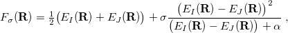
where  is a fixed parameter to avoid singularities and
  is a Lagrange multiplier for a penalty function meant to drive the energy gap to zero. Optimization of
  proceeds iteratively for increasingly large values of the parameter . The second MECP optimization algorithm is a simplification of the first one that we call the “direct” method. Here, the gradient of the objective function is
 |
(9.5) |
where
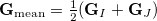 |
(9.6) |
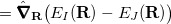
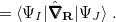
is the mean energy gradient (with  being the nuclear gradient for state
  ), and
 |
(9.7) |
is the normalized difference gradient. Finally,
 |
(9.8) |
projects the gradient difference direction out of the mean energy gradient in Eq. eq:direct_MECP. The third and final MECP optimization algorithm that is available in Q-Chem is the branching-plane updating method developed by Maeda et al. [418]. This algorithm uses a gradient that is similar to that in Eq. eq:direct_MECP but projects out not just  in Eq. eq:MECP_projector but also a second vector that is orthogonal to it.
None of these three methods requires evaluation of nonadiabatic couplings, and all three can be used to optimize MECPs at the CIS, SF-CIS, TDDFT, SF-TDDFT, and SOS-CIS(D0) levels. The direct algorithm can also be used for EOM-XX-CCSD methods. Note, however, that all linear-response methods (a category that includes CIS, TDDFT, and EOM-XX-CCSD) incorrectly describe the topology of any conical intersection that involves the reference (usually, ground) state. Specifically, it can be shown in such cases that only a one-dimensional branching space is obtained [419]. If conical intersections involving the ground state are to be described correctly, one must use a different reference state, which can be accomplished with spin-flip (SF) methods [420, 421, 422]. In particular, using a high-spin triplet reference state, the ground-state singlet ( ) appears as an excitation (possibly with a negative excitation energy) alongside the excited-state singlets,
  , so there is no topology problem in describing an /
 conical intersection. Accurate MECP geometries, as compared to multireference configuration-interaction benchmarks, have been reported [421]. It should be noted, however, that the
  component of the triplet state also shows up as an excitation in SF methods, and while Q-Chem attempts to identify this triplet state automatically (based on a threshold for
  ), severe spin contamination can sometimes hamper one’s ability to distinguish this state from the singlet excited states [421].
In Q-Chem 4.3, analytic derivative couplings for CIS and TDDFT have been implemented 10.3. Thus, CIS and TDDFT MECP optimizations can use this new feature to reduce the optimization cycles.[422] Note that the $derivative_coupling section is not required in MECP optimization jobs, and $rem variable MECP_METHODS must be set to BRANCHING_PLANE.
9.4.1 Job Control
MECP_OPT
Determines whether we are doing MECP optimizations.
TYPE:
LOGICAL
DEFAULT:
FALSE
OPTIONS:
TRUE
Do MECP optimizations.
FALSE
Don’t do MECP optimizations.
RECOMMENDATION:
None.
MECP_METHODS
Determines which method to be used.
TYPE:
STRING
DEFAULT:
BRANCHING_PLANE
OPTIONS:
BRANCHING_PLANE
Use the branching-plane updating method.
MECP_DIRECT
Use the direct method.
PENALTY_FUNCTION
Use the penalty-constrained method.
RECOMMENDATION:
The direct method is stable for small molecules or molecules with high symmetries, but the branching-plane updating method is more efficient for larger molecules. However, the latter does not work if the two states have different symmetries. If using branching plane updating method, GEOM_OPT_COORDS must be set to 0 in the $rem section (i.e., this algorithm is available in Cartesian coordinates only). The penalty-constrained method converges slowly and is suggested only when the other methods do not work.
MECP_STATE1
Determines the first state for crossing.
TYPE:
INTEGER/INTEGER ARRAY
DEFAULT:
None
OPTIONS:
[
]
find the
means the SCF ground state.
RECOMMENDATION:
MECP_STATE2
Determines the second state for crossing.
TYPE:
INTEGER/INTEGER ARRAY
DEFAULT:
None
OPTIONS:
[
find the
RECOMMENDATION:
CIS_S2_THRESH
Determines whether a state is singlet or triplet in unrestricted calculations.
TYPE:
INTEGER
DEFAULT:
120
OPTIONS:
None
RECOMMENDATION:
If set to 120, the states with
are treated as triplet states, with other states are treated as singlets.
MECP_PROJ_HESS
Determines whether to project out the coupling vector from the Hessian when using branching plane updating method.
TYPE:
LOGICAL
DEFAULT:
TRUE
OPTIONS:
TRUE
FALSE
RECOMMENDATION:
Use Default.
9.4.2 Examples
The MECP between the S and S
and S states of NO
 is optimized using the direct method:
Example 9.192 MECP optimization for NO using SOS-CIS(D0)
$MOLECULE
-1 1
N1
O2 N1 RNO
O3 N1 RNO O2 AONO

RNO=1.50
AONO=100
$END

$rem
  jobtype         = opt
  method          = soscis(d0)
  basis           = aug-cc-pVDZ
  aux_basis       = rimp2-aug-cc-pVDZ
  purecart        = 1111
  cis_n_roots     = 4
  cis_triplets    = false
  cis_singlets    = true
  mem_static      = 900
  mem_total       = 1950
  mecp_opt true
  mecp_state1 [0,2]
  mecp_state2 [0,3]
  mecp_methods mecp_direct
$end
The MECP between the S and S
and S states of ethylidene is optimized using the branching-plane update method:
Example 9.193 MECP optimization for ethylidene using SF-TDDFT
$molecule
0 3
C  0.0446266041 -0.2419241370 0.3571573801
C  0.0089051507 0.6727548956 1.4605006396
H  0.9284257388 -0.1459163900 -0.2720952334
H -0.8310326564 -0.1926895078 -0.2885298629
H -0.0092388670 0.9611331703 2.4799363398
H  0.0683140308 -1.2533580302 0.7788470826
$end

$rem
jobtype       opt
mecp_opt      true
mecp_methods  branching_plane
MECP_PROJ_HESS true !project out y vector from the hessian
GEOM_OPT_COORDS 0  !currently only works for Cartesian coordinate

method        bhhlyp
spin_flip     true
unrestricted  true
basis         6-31G(d,p)
cis_n_roots   4
mecp_state1   [0,1]
mecp_state2   [0,2]
CIS_S2_THRESH 120
$end
The MECP between S and S states of twisted-pyramidalized ethylene is optimized using the penalty-constrained method:
Example 9.194 MECP optimization for ethylene using SF-TDDFT
$molecule
0 3
C -0.0158897609 0.0735325545 -0.0595597308
C  0.0124274563 -0.0024687284 1.3156941918
H  0.8578762360 0.1470146857 -0.7105293671
H -0.9364708648 -0.0116961121 -0.6267613144
H  0.7645577838 0.6633816890 1.7625731128
H  0.7407739370 -0.8697640880 1.3285831079
$end

$rem
jobtype       opt
mecp_opt      true
mecp_methods  PENALTY_FUNCTION

method        bhhlyp
spin_flip     true
unrestricted  true
basis         6-31G(d,p)
cis_n_roots   4
mecp_state1   [0,1]
mecp_state2   [0,2]
CIS_S2_THRESH 120
$end
The MECP between 
 A and ÃB states of the N
 ion using the direct method:
Example 9.195 MECP optimization for N using EOM-EE-CCSD
$MOLECULE
1 1
N1
N2 N1 rNN
N3 N2 rNN N1 aNNN

rNN=1.54
aNNN=50.0
$END

$REM
JOBTYPE               OPT
MECP_OPT              TRUE
MECP_METHODS          mecp_direct

METHOD                EOM-CCSD
BASIS                 6-31G

ee_singlets           [0,2,0,2]

XOPT_STATE_1          [0,2,2]
XOPT_STATE_2          [0,4,1]
ccman2                false

GEOM_OPT_TOL_GRADIENT 30
$END
MECP optimization using analytic derivative coupling:
Example 9.196 MECP between and of ethylidene optimized using BH&HLYP spin-flip TDDFT with analytic derivative coupling
$molecule
0 3
C  0.0446266041 -0.2419241370 0.3571573801
C  0.0089051507 0.6727548956 1.4605006396
H  0.9284257388 -0.1459163900 -0.2720952334
H -0.8310326564 -0.1926895078 -0.2885298629
H -0.0092388670 0.9611331703 2.4799363398
H  0.0683140308 -1.2533580302 0.7788470826
$end

$rem
jobtype opt
mecp_opt      true
mecp_methods  branching_plane
MECP_PROJ_HESS true
GEOM_OPT_COORDS 0
mecp_state1  [0,1]
mecp_state2  [0,2]
unrestricted true
spin_flip true
cis_n_roots 4
cis_der_couple true
CIS_DER_NUMSTATE 2
set_iter 50
exchange bhhlyp
basis 6-31G(d,p)
symmetry_ignore true
$end