4.9 Constrained Density Functional Theory (CDFT)

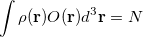
Under certain circumstances, it is desirable to apply constraints to the electron density during a self-consistent calculation. For example, in a transition metal complex it may be desirable to constrain the net spin density on a particular metal atom to integrate to a value consistent with the $M_ S$ value expected from ligand field theory. Similarly, in a donor-acceptor complex one may be interested in constraining the total density on the acceptor group so that the formal charge on the acceptor is either neutral or negatively charged, depending as the molecule is in its neutral or charge transfer configuration. In these situations, one is interested in controlling the average value of some density observable, $O(\mathbf{r})$ , to take on a given value, $N$ :

$\begin{equation} \int \rho (\mathbf{r}) O(\mathbf{r}) d^3\mathbf{r} = N \end{equation}$

(4.96)

There are of course many states that satisfy such a constraint, but in practice one is usually looking for the lowest energy such state. To solve the resulting constrained minimization problem, one introduces a Lagrange multiplier, $V$ , and solves for the stationary point of

$\begin{equation} V[\rho , V] = E[\rho ] - V(\int \rho (\mathbf{r}) O(\mathbf{r}) d^3\mathbf{r} - N ) \end{equation}$

(4.97)

where $E[\rho ]$ is the energy of the system described using density functional theory (DFT). At convergence, the functional $W$ gives the density, $\rho$ , that satisfies the constraint exactly (i.e., it has exactly the prescribed number of electrons on the acceptor or spins on the metal center) but has the lowest energy possible. The resulting self-consistent procedure can be efficiently solved by ensuring at every SCF step the constraint is satisfied exactly. The Q-Chem implementation of these equations closely parallels those in Ref. Wu:2005.

The first step in any constrained DFT calculation is the specification of the constraint operator, $O(\mathbf{r})$ . Within Q-Chem, the user is free to specify any constraint operator that consists of a linear combination of the Becke’s atomic partitioning functions:

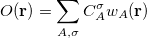$\begin{equation} O(\mathbf{r}) = \sum _{A,\sigma } C^{\sigma }_ A w_ A(\mathbf{r}) \end{equation}$

(4.98)

Here the summation runs over the atoms in the system ( $A$ ) and over the electron spin ( $\sigma = \alpha , \beta$ ). Note that each weight function is designed to be nearly 1 near the nucleus of atom $A$ and rapidly fall to zero near the nucleus of any other atom in the system. The specification of the $C_ A^{\sigma }$ coefficients is accomplished using

$cdft
CONSTRAINT_VALUE_X
COEFFICIENT1_X       FIRST_ATOM1_X       LAST_ATOM1_X    TYPE1_X
COEFFICIENT2_X       FIRST_ATOM2_X       LAST_ATOM2_X    TYPE2_X
...
CONSTRAINT_VALUE_Y
COEFFICIENT1_Y       FIRST_ATOM1_Y       LAST_ATOM1_Y    TYPE1_Y
COEFFICIENT2_Y       FIRST_ATOM2_Y       LAST_ATOM2_Y    TYPE2_Y
...
...
$end

Here, each CONSTRAINT_VALUE is a real number that specifies the desired average value ( $N$ ) of the ensuing linear combination of atomic partition functions. Each COEFFICIENT specifies the coefficient ( $C_{\alpha }$ ) of a partition function or group of partition functions in the constraint operator $O$ . For each coefficient, all the atoms between the integers FIRST_ATOM and LAST_ATOM contribute with the specified weight in the constraint operator. Finally, TYPE specifies the type of constraint being applied—either “CHARGE” or “SPIN”. For a CHARGE constraint the spin up and spin down densities contribute equally ( $C_ A^{\alpha }=C_ A^{\beta } = C_ A$ ) yielding the total number of electrons on the atom A. For a SPIN constraint, the spin up and spin down densities contribute with opposite sign ( $C_ A^{\alpha }-C_ A^{\beta } = C_ A$ ) resulting in a measure of the net spin on the atom A. Each separate CONSTRAINT_VALUE creates a new operator whose average is to be constrained—for instance, the example above includes several independent constraints: $\rm X, Y, \ldots$ . Q-Chem can handle an arbitrary number of constraints and will minimize the energy subject to all of these constraints simultaneously.

In addition to the $cdft input section of the input file, a constrained DFT calculation must also set the CDFT flag to TRUE for the calculation to run. If an atom is not included in a particular operator, then the coefficient of that atoms partition function is set to zero for that operator. The TYPE specification is optional, and the default is to perform a charge constraint. Further, note that any charge constraint is on the net atomic charge. That is, the constraint is on the difference between the average number of electrons on the atom and the nuclear charge. Thus, to constrain CO to be negative, the constraint value would be 1 and not 15.

Note: Charge constraint in $cdft specifies the number of excess electrons on a fragment, not the total charge, i.e., the value 1.0 means charge=-1, whereas charge constraint of -1.0 corresponds to the total +1 charge.

The choice of which atoms to include in different constraint regions is left entirely to the user and in practice must be based somewhat on chemical intuition. Thus, for example, in an electron transfer reaction the user must specify which atoms are in the “donor” and which are in the “acceptor”. In practice, the most stable choice is typically to make the constrained region as large as physically possible. Thus, for the example of electron transfer again, it is best to assign every atom in the molecule to one or the other group (donor or acceptor), recognizing that it makes no sense to assign any atoms to both groups. On the other end of the spectrum, constraining the formal charge on a single atom is highly discouraged. The problem is that while our chemical intuition tells us that the lithium atom in LiF should have a formal charge of +1, in practice the quantum mechanical charge is much closer to +0.5 than +1. Only when the fragments are far enough apart do our intuitive pictures of formal charge actually become quantitative.

Note that the atomic populations that Q-Chem prints out are Mulliken populations, not the Becke weights populations. As a result, the printed populations will not generally add up to the specified constrained values, even though the constraint is exactly satisfied. You can print Becke populations to confirm that the computed states have the desired charge/spin character.

Finally, we note that SCF convergence is typically more challenging in constrained DFT calculations as compared to their unconstrained counterparts. This effect arises because applying the constraint typically leads to a broken symmetry, diradical-like state. As SCF convergence for these cases is known to be difficult even for unconstrained states, it is perhaps not surprising that there are additional convergence difficulties in this case. Please see the section on SCF convergence for ideas on how to improve convergence for constrained calculations. Also, CDFT is more sensitive to grid size than ground-state DFT, so sometimes upping the integration grid to (50,194) or (75, 302) improves the convergence.

Note: To improve convergence, use the fewest possible constraints. For example, if your system consists of two fragments, specify the constrains for one of them only. The overall charge and multiplicity will force the "unconstrained" fragment to attain the right charge and multiplicity.

Note: The direct minimization methods are not available for constrained calculations. Hence, some combination of DIIS and RCA must be used to obtain convergence. Further, it is often necessary to break symmetry in the initial guess (using SCF_GUESS_MIX) to ensure that the lowest energy solution is obtained.

Analytic gradients are available for constrained DFT calculations [214]. Second derivatives are only available by finite difference of gradients. For details on how to apply constrained DFT to compute magnetic exchange couplings, see Ref. Wu:2006b. For details on using constrained DFT to compute electron transfer parameters, see Ref. Wu:2006c.

CDFT options are:

CDFT

Initiates a constrained DFT calculation

TYPE:

LOGICAL

DEFAULT:

FALSE

OPTIONS:

TRUE

Perform a Constrained DFT Calculation

FALSE

No Density Constraint

RECOMMENDATION:

Set to TRUE if a Constrained DFT calculation is desired.

CDFT_POSTDIIS

Controls whether the constraint is enforced after DIIS extrapolation.

TYPE:

LOGICAL

DEFAULT:

TRUE

OPTIONS:

TRUE

Enforce constraint after DIIS

FALSE

Do not enforce constraint after DIIS

RECOMMENDATION:

Use default unless convergence problems arise, in which case it may be beneficial to experiment with setting CDFT_POSTDIIS to FALSE. With this option set to TRUE, energies should be variational after the first iteration.

CDFT_PREDIIS

Controls whether the constraint is enforced before DIIS extrapolation.

TYPE:

LOGICAL

DEFAULT:

FALSE

OPTIONS:

TRUE

Enforce constraint before DIIS

FALSE

Do not enforce constraint before DIIS

RECOMMENDATION:

Use default unless convergence problems arise, in which case it may be beneficial to experiment with setting CDFT_PREDIIS to TRUE. Note that it is possible to enforce the constraint both before and after DIIS by setting both CDFT_PREDIIS and CDFT_POSTDIIS to TRUE.

CDFT_THRESH

Threshold that determines how tightly the constraint must be satisfied.

TYPE:

INTEGER

DEFAULT:

5

OPTIONS:

N

Constraint is satisfied to within $10^{-N}$ .

RECOMMENDATION:

Use default unless problems occur.

CDFT_CRASHONFAIL

Whether the calculation should crash or not if the constraint iterations do not converge.

TYPE:

LOGICAL

DEFAULT:

TRUE

OPTIONS:

TRUE

Crash if constraint iterations do not converge.

FALSE

Do not crash.

RECOMMENDATION:

Use default.

CDFT_BECKE_POP

Whether the calculation should print the Becke atomic charges at convergence

TYPE:

LOGICAL

DEFAULT:

TRUE

OPTIONS:

TRUE

Print Populations

FALSE

Do not print them

RECOMMENDATION:

Use default. Note that the Mulliken populations printed at the end of an SCF run will not typically add up to the prescribed constraint value. Only the Becke populations are guaranteed to satisfy the user-specified constraints.

Example 4.74 Charge separation on FAAQ

$molecule
0 1
 C     -0.64570736     1.37641945    -0.59867467
 C      0.64047568     1.86965826    -0.50242683
 C      1.73542663     1.01169939    -0.26307089
 C      1.48977850    -0.39245666    -0.15200261
 C      0.17444585    -0.86520769    -0.27283957
 C     -0.91002699    -0.02021483    -0.46970395
 C      3.07770780     1.57576311    -0.14660056
 C      2.57383948    -1.35303134     0.09158744
 C      3.93006075    -0.78485926     0.20164558
 C      4.16915637     0.61104948     0.08827557
 C      5.48914671     1.09087541     0.20409492
 H      5.64130588     2.16192921     0.11315072
 C      6.54456054     0.22164774     0.42486947
 C      6.30689287    -1.16262761     0.53756193
 C      5.01647654    -1.65329553     0.42726664
 H     -1.45105590     2.07404495    -0.83914389
 H      0.85607395     2.92830339    -0.61585218
 H      0.02533661    -1.93964850    -0.19096085
 H      7.55839768     0.60647405     0.51134530
 H      7.13705743    -1.84392666     0.71043613
 H      4.80090178    -2.71421422     0.50926027
 O      2.35714021    -2.57891545     0.20103599
 O      3.29128460     2.80678842    -0.23826460
 C     -2.29106231    -0.63197545    -0.53957285
 O     -2.55084900    -1.72562847    -0.95628300
 N     -3.24209015     0.26680616     0.03199109
 H     -2.81592456     1.08883943     0.45966550
 C     -4.58411403     0.11982669     0.15424004
 C     -5.28753695     1.14948617     0.86238753
 C     -5.30144592    -0.99369577    -0.39253179
 C     -6.65078185     1.06387425     1.01814801
 H     -4.73058059     1.98862544     1.26980479
 C     -6.66791492    -1.05241167    -0.21955088
 H     -4.76132422    -1.76584307    -0.92242502
 C     -7.35245187    -0.03698606     0.47966072
 H     -7.18656323     1.84034269     1.55377875
 H     -7.22179827    -1.89092743    -0.62856041
 H     -8.42896369    -0.10082875     0.60432214
$end

$rem
JOBTYPE         FORCE
METHOD          B3LYP
BASIS           6-31G*
SCF_PRINT       TRUE
CDFT            TRUE
$end

$cdft
2
 1 1  25
-1 26 38
$end

Example 4.75 Cu2-Ox High Spin

$molecule
2 3
 Cu      1.4674     1.6370     1.5762
 O       1.7093     0.0850     0.3825
 O      -0.5891     1.3402     0.9352
 C       0.6487    -0.3651    -0.1716
 N       1.2005     3.2680     2.7240
 N       3.0386     2.6879     0.6981
 N       1.3597     0.4651     3.4308
 H       2.1491    -0.1464     3.4851
 H       0.5184    -0.0755     3.4352
 H       1.3626     1.0836     4.2166
 H       1.9316     3.3202     3.4043
 H       0.3168     3.2079     3.1883
 H       1.2204     4.0865     2.1499
 H       3.8375     2.6565     1.2987
 H       3.2668     2.2722    -0.1823
 H       2.7652     3.6394     0.5565
 Cu     -1.4674    -1.6370    -1.5762
 O      -1.7093    -0.0850    -0.3825
 O       0.5891    -1.3402    -0.9352
 C      -0.6487     0.3651     0.1716
 N      -1.2005    -3.2680    -2.7240
 N      -3.0386    -2.6879    -0.6981
 N      -1.3597    -0.4651    -3.4308
 H      -2.6704    -3.4097    -0.1120
 H      -3.6070    -3.0961    -1.4124
 H      -3.5921    -2.0622    -0.1485
 H      -0.3622    -3.1653    -3.2595
 H      -1.9799    -3.3721    -3.3417
 H      -1.1266    -4.0773    -2.1412
 H      -0.5359     0.1017    -3.4196
 H      -2.1667     0.1211    -3.5020
 H      -1.3275    -1.0845    -4.2152
$end

$rem
JOBTYPE         SP
METHOD          B3LYP
BASIS           6-31G*
SCF_PRINT       TRUE
CDFT            TRUE
$end

$cdft
2
 1 1   3  s
-1 17 19  s
$end

TRUE	Perform a Constrained DFT Calculation
FALSE	No Density Constraint

TRUE	Enforce constraint after DIIS
FALSE	Do not enforce constraint after DIIS

TRUE	Enforce constraint before DIIS
FALSE	Do not enforce constraint before DIIS

TRUE	Crash if constraint iterations do not converge.
FALSE	Do not crash.