5.14 Simplified Coupled-Cluster Methods Based on a Perfect-Pairing Active Space
The methods described below are related to valence bond theory and are handled by the GVBMAN module. The following models are available:
CORRELATION
Specifies the correlation level in GVB models handled by GVBMAN.
TYPE:
STRING
DEFAULT:
None
No Correlation
OPTIONS:
PP
CCVB
GVB_IP
GVB_SIP
GVB_DIP
OP
NP
2P
RECOMMENDATION:
As a rough guide, use PP for biradicaloids, and CCVB for polyradicaloids involving strong spin correlations. Consult the literature for further guidance.
Molecules where electron correlation is strong are characterized by small energy gaps between the nominally occupied orbitals (that would comprise the Hartree-Fock wave function, for example) and nominally empty orbitals. Examples include so-called diradicaloid molecules [316], or molecules with partly broken chemical bonds (as in some transition-state structures). Because the energy gap is small, electron configurations other than the reference determinant contribute to the molecular wave function with considerable amplitude, and omitting them leads to a significant error.
Including all possible configurations however, is a vast overkill. It is common to restrict the configurations that one generates to be constructed not from all molecular orbitals, but just from orbitals that are either “core” or “active”. In this section, we consider just one type of active space, which is composed of two orbitals to represent each electron pair: one nominally occupied (bonding or lone pair in character) and the other nominally empty, or correlating (it is typically antibonding in character). This is usually called the perfect pairing active space, and it clearly is well-suited to represent the bonding-antibonding correlations that are associated with bond-breaking.
The quantum chemistry within this (or any other) active space is given by a Complete Active Space SCF (CASSCF) calculation, whose exponential cost growth with molecule size makes it prohibitive for systems with more than about 14 active orbitals. One well-defined coupled cluster (CC) approximation based on CASSCF is to include only double substitutions in the valence space whose orbitals are then optimized. In the framework of conventional CC theory, this defines the valence optimized doubles (VOD) model [308], which scales as  (see Section 5.9.2). This is still too expensive to be readily applied to large molecules.
The methods described in this section bridge the gap between sophisticated but expensive coupled cluster methods and inexpensive methods such as DFT, HF and MP2 theory that may be (and indeed often are) inadequate for describing molecules that exhibit strong electron correlations such as diradicals. The coupled cluster perfect pairing (PP) [317, 318], imperfect pairing (IP) [319] and restricted coupled cluster (RCC) [320] models are local approximations to VOD that include only a linear and quadratic number of double substitution amplitudes respectively. They are close in spirit to generalized valence bond (GVB)-type wave functions [321], because in fact they are all coupled cluster models for GVB that share the same perfect pairing active space. The most powerful method in the family, the Coupled Cluster Valence Bond (CCVB) method [322, 323, 324], is a valence bond approach that goes well beyond the power of GVB-PP and related methods, as discussed below in Sec. 5.14.2.
5.14.1 Perfect pairing (PP)
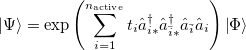
To be more specific, the coupled cluster PP wave function is written as
 |
(5.42) |
where  is the number of active electrons, and the
  are the linear number of unknown cluster amplitudes, corresponding to exciting the two electrons in the
  th electron pair from their bonding orbital pair to their antibonding orbital pair. In addition to , the core and the active orbitals are optimized as well to minimize the PP energy. The algorithm used for this is a slight modification of the GDM method, described for SCF calculations in Section 4.6.4. Despite the simplicity of the PP wave function, with only a linear number of correlation amplitudes, it is still a useful theoretical model chemistry for exploring strongly correlated systems. This is because it is exact for a single electron pair in the PP active space, and it is also exact for a collection of non-interacting electron pairs in this active space. Molecules, after all, are in a sense a collection of interacting electron pairs! In practice, PP on molecules recovers between 60% and 80% of the correlation energy in its active space.
If the calculation is perfect pairing (CORRELATION = PP), it is possible to look for unrestricted solutions in addition to restricted ones. Unrestricted orbitals are the default for molecules with odd numbers of electrons, but can also be specified for molecules with even numbers of electrons. This is accomplished by setting GVB_UNRESTRICTED = TRUE. Given a restricted guess, this will, however usually converge to a restricted solution anyway, so additional REM variables should be specified to ensure an initial guess that has broken spin symmetry. This can be accomplished by using an unrestricted SCF solution as the initial guess, using the techniques described in Chapter 4. Alternatively a restricted set of guess orbitals can be explicitly symmetry broken just before the calculation starts by using GVB_GUESS_MIX, which is described below. There is also the implementation of Unrestricted-in-Active Pairs (UAP) [325] which is the default unrestricted implementation for GVB methods. This method simplifies the process of unrestriction by optimizing only one set of ROHF MO coefficients and a single rotation angle for each occupied-virtual pair. These angles are used to construct a series of 2x2 Given’s rotation matrices which are applied to the ROHF coefficients to determine the  spin MO coefficients and their transpose is applied to the ROHF coefficients to determine the
  spin MO coefficients. This algorithm is fast and eliminates many of the pathologies of the unrestricted GVB methods near the dissociation limit. To generate a full potential curve we find it is best to start at the desired UHF dissociation solution as a guess for GVB and follow it inwards to the equilibrium bond distance.
GVB_UNRESTRICTED
Controls restricted versus unrestricted PP jobs. Usually handled automatically.
TYPE:
LOGICAL
DEFAULT:
same value as UNRESTRICTED
OPTIONS:
TRUE/FALSE
RECOMMENDATION:
Set this variable explicitly only to do a UPP job from an RHF or ROHF initial guess. Leave this variable alone and specify UNRESTRICTED=TRUE to access the new Unrestricted-in-Active-Pairs GVB code which can return an RHF or ROHF solution if used with GVB_DO_ROHF
GVB_DO_ROHF
Sets the number of Unrestricted-in-Active Pairs to be kept restricted.
TYPE:
INTEGER
DEFAULT:
0
OPTIONS:

User-Defined
RECOMMENDATION:
If
GVB_OLD_UPP
Which unrestricted algorithm to use for GVB.
TYPE:
INTEGER
DEFAULT:
0
OPTIONS:
0
Use Unrestricted-in-Active Pairs described in Ref. Lawler:2010
1
Use Unrestricted Implementation described in Ref. Beran:2005
RECOMMENDATION:
Only works for Unrestricted PP and no other GVB model.
GVB_GUESS_MIX
Similar to SCF_GUESS_MIX, it breaks alpha/beta symmetry for UPP by mixing the alpha HOMO and LUMO orbitals according to the user-defined fraction of LUMO to add the HOMO. 100 corresponds to a 1:1 ratio of HOMO and LUMO in the mixed orbitals.
TYPE:
INTEGER
DEFAULT:
0
OPTIONS:
User-defined,

RECOMMENDATION:
25 often works well to break symmetry without overly impeding convergence.
Whilst all of the description in this section refers to PP solved projectively, it is also possible, as described in Sec. 5.14.2 below, to solve variationally for the PP energy. This variational PP solution is the reference wave function for the CCVB method. In most cases use of spin-pure CCVB is preferable to attempting to improve restricted PP by permitting the orbitals to spin polarize.
5.14.2 Coupled Cluster Valence Bond (CCVB)
Cases where PP needs improvement include molecules with several strongly correlated electron pairs that are all localized in the same region of space, and therefore involve significant inter-pair, as well as intra-pair correlations. For some systems of this type, Coupled Cluster Valence Bond (CCVB) [322, 323] is an appropriate method. CCVB is designed to qualitatively treat the breaking of covalent bonds. At the most basic theoretical level, as a molecular system dissociates into a collection of open-shell fragments, the energy should approach the sum of the ROHF energies of the fragments. CCVB is able to reproduce this for a wide class of problems, while maintaining proper spin symmetry. Along with this, CCVB’s main strength, come many of the spatial symmetry breaking issues common to the GVB-CC methods.
Like the other methods discussed in this section, the leading contribution to the CCVB wave function is the perfect pairing wave function, which is shown in eqn. eqn:PP. One important difference is that CCVB uses the PP wave function as a reference in the same way that other GVBMAN methods use a reference determinant.
The PP wave function is a product of simple, strongly orthogonal singlet geminals. Ignoring normalizations, two equivalent ways of displaying these geminals are
 |
|||
 |
(5.43) |
where on the left and right we have the spatial part (involving  and
and  orbitals) and the spin coupling, respectively. The VB-form orbitals are non-orthogonal within a pair and are generally AO-like. The VB form is used in CCVB and the NO form is used in the other GVBMAN methods. It turns out that occupied UHF orbitals can also be rotated (without affecting the energy) into the VB form (here the spin part would be just
  ), and as such we store the CCVB orbital coefficients in the same way as is done in UHF (even though no one spin is assigned to an orbital in CCVB).
These geminals are uncorrelated in the same way that molecular orbitals are uncorrelated in a HF calculation. Hence, they are able to describe uncoupled, or independent, single-bond-breaking processes, like that found in C H
H
 2 CH
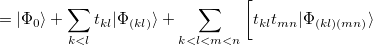
2 CH , but not coupled multiple-bond-breaking processes, such as the dissociation of N. In the latter system the three bonds may be described by three singlet geminals, but this picture must somehow translate into the coupling of two spin-quartet N atoms into an overall singlet, as found at dissociation. To achieve this sort of thing in a GVB context, it is necessary to correlate the geminals. The part of this correlation that is essential to bond breaking is obtained by replacing clusters of singlet geminals with triplet geminals, and recoupling the triplets to an overall singlet. A triplet geminal is obtained from a singlet by simply modifying the spin component accordingly. We thus obtain the CCVB wave function:
 |
 |
|||
 |
![$\displaystyle + t_{km} t_{ln} |\Phi _{(km)(ln)}\rangle + t_{kn} t_{lm} |\Phi _{(kn)(lm)}\rangle \bigg] + \cdots . $](images/img-0629.png) |
(5.44) |
In this expansion, the summations go over the active singlet pairs, and the indices shown in the labellings of the kets correspond to pairs that are being coupled as described just above. We see that this wave function couples clusters composed of even numbers of geminals. In addition, we see that the amplitudes for clusters containing more than 2 geminals are parameterized by the amplitudes for the 2-pair clusters. This approximation is important for computational tractability, but actually is just one in a family of CCVB methods: it is possible to include coupled clusters of odd numbers of pairs, and also to introduce independent parameters for the higher-order amplitudes. At present, only the simplest level is included in Q-Chem.
Older methods which attempt to describe substantially the same electron correlation effects as CCVB are the IP [319] and RCC [320] wave functions. In general CCVB should be used preferentially. It turns out that CCVB relates to the GVB-IP model. In fact, if we were to expand the CCVB wave function relative to a set of determinants, we would see that for each pair of singlet pairs, CCVB contains only one of the two pertinent GVB-IP doubles amplitudes. Hence, for CCVB the various computational requirements and timings are very similar to those for GVB-IP. The main difference between the two models lies in how the doubles amplitudes are used to parameterize the quadruples, sextuples, etc., and this is what allows CCVB to give correct energies at full bond dissociation.
A CCVB calculation is invoked by setting CORRELATION = CCVB. The number of active singlet geminals must be specified by GVB_N_PAIRS. After this, an initial guess is chosen. There are three main options for this, specified by the following keyword
CCVB_GUESS
Specifies the initial guess for CCVB calculations
TYPE:
INTEGER
DEFAULT:
NONE
OPTIONS:
1
Standard GVBMAN guess (orbital localization via GVB_LOCAL + Sano procedure).
2
Use orbitals from previous GVBMAN calculation, along with SCF_GUESS = read.
3
Convert UHF orbitals into pairing VB form.
RECOMMENDATION:
Option 1 is the most useful overall. The success of GVBMAN methods is often dependent on localized orbitals, and this guess shoots for these. Option 2 is useful for comparing results to other GVBMAN methods, or if other GVBMAN methods are able to obtain a desired result more efficiently. Option 3 can be useful for bond-breaking situations when a pertinent UHF solution has been found. It works best for small systems, or if the unrestriction is a local phenomenon within a larger molecule. If the unrestriction is non-local and the system is large, this guess will often produce a solution that is not the global minimum. Any UHF solution has a certain number of pairs that are unrestricted, and this will be output by the program. If GVB_N_PAIRS exceeds this number, the standard GVBMAN initial-guess procedure will be used to obtain a guess for the excess pairs
For potential energy surfaces, restarting from a previously computed CCVB solution is recommended. This is invoked by GVB_RESTART = TRUE. Whenever this is used, or any time orbitals are being read directly into CCVB from another calculation, it is important to also set:
SCF_GUESS = READ
MP2_RESTART_NO_SCF = TRUE
SCF_ALGORITHM = DIIS
This bypasses orthogonalization schemes used elsewhere within Q-Chem that are likely to jumble the CCVB guess.
In addition to the parent CCVB method as discussed up until now, we have included two related schemes for energy optimization, whose operation is controlled by the following keyword:
CCVB_METHOD
Optionally modifies the basic CCVB method
TYPE:
INTEGER
DEFAULT:
1
OPTIONS:
1
Standard CCVB model
3
Independent electron pair approximation (IEPA) to CCVB
4
Variational PP (the CCVB reference energy)
RECOMMENDATION:
Option 1 is generally recommended. Option 4 is useful for preconditioning, and for obtaining localized-orbital solutions, which may be used in subsequent calculations. It is also useful for cases in which the regular GVBMAN PP code becomes variationally unstable. Option 3 is a simple independent-amplitude approximation to CCVB. It avoids the cubic-scaling amplitude equations of CCVB, and also is able to reach the correct dissociation energy for any molecular system (unlike regular CCVB which does so only for cases in which UHF can reach a correct dissociate limit). However the IEPA approximation to CCVB is sometimes variationally unstable, which we have yet to observe in regular CCVB.
Example 5.94 N molecule in the intermediately dissociated region. In this case, SCF_ALGORITHM DIIS is necessary to obtain the symmetry unbroken RHF solution, which itself is necessary to obtain the proper CCVB solution. Note that many keywords general to GVBMAN are also used in CCVB.
$molecule
  0 1
  N 0 0 0
  N 0 0 2.0
$end

$rem
  jobtype            = sp
  unrestricted       = false
  basis              = 6-31g*
  exchange           = hf
  correlation        = ccvb
  gvb_n_pairs        = 3
  ccvb_method        = 1
  ccvb_guess         = 1
  gvb_local          = 2
  gvb_orb_max_iter   = 100000
  gvb_orb_conv       = 7
  gvb_restart        = false
  scf_convergence    = 10
  thresh             = 14
  scf_guess          = sad
  mp2_restart_no_scf = false
  scf_algorithm      = diis
  max_scf_cycles     = 2000
  symmetry           = false
  sym_ignore         = true
  print_orbitals     = true
$end
5.14.3 Second order correction to perfect pairing: PP(2)
The PP and CCVB models are potential replacements for HF theory as a zero order description of electronic structure and can be used as a starting point for perturbation theory. They neglect all correlations that involve electron configurations with one or more orbitals that are outside the active space. Physically this means that the so-called “dynamic correlations”, which correspond to atomic-like correlations involving high angular momentum virtual levels are neglected. Therefore, the GVB models may not be very accurate for describing energy differences that are sensitive to this neglected correlation energy, e.g., atomization energies. It is desirable to correct them for this neglected correlation in a way that is similar to how the HF reference is corrected via MP2 perturbation theory.
For this purpose, the leading (second order) correction to the PP model, termed PP(2) [326], has been formulated and efficiently implemented for restricted and unrestricted orbitals (energy only). PP(2) improves upon many of the worst failures of MP2 theory (to which it is analogous), such as for open shell radicals. PP(2) also greatly improves relative energies relative to PP itself. PP(2) is implemented using a resolution of the identity (RI) approach to keep the computational cost manageable. This cost scales in the same 5th-order way with molecular size as RI-MP2, but with a pre-factor that is about 5 times larger. It is therefore vastly cheaper than CCSD or CCSD(T) calculations which scale with the 6th and 7th powers of system size respectively. PP(2) calculations are requested with CORRELATION = PP(2). Since the only available algorithm uses auxiliary basis sets, it is essential to also provide a valid value for AUX_BASIS to have a complete input file.
The example below shows a PP(2) input file for the challenging case of the N2 molecule with a stretched bond. For this reason a number of the non-standard options discussed in Sec. 5.14.1 and Sec. 5.14.4 for orbital convergence are enabled here. First, this case is an unrestricted calculation on a molecule with an even number of electrons, and so it is essential to break the alpha/beta spin symmetry in order to find an unrestricted solution. Second, we have chosen to leave the lone pairs uncorrelated, which is accomplished by specifying GVB_N_PAIRS.
Example 5.95 A non-standard PP(2) calculation. UPP(2) for stretched N2 with only 3 correlating pairs Try Boys localization scheme for initial guess.
$molecule
   0 1
   N
   N   1   1.65
$end

$rem
   UNRESTRICTED    true
   CORRELATION     pp(2)
   EXCHANGE        hf
   BASIS           cc-pvdz
   AUX_BASIS       rimp2-cc-pvdz   must use RI with PP(2)
%   PURECART        11111
   SCF_GUESS_MIX   10              mix SCF guess 100{\%}
   GVB_GUESS_MIX   25              mix GVB guess 25{\%} also!
   GVB_N_PAIRS     3               correlate only 3 pairs
   GVB_ORB_CONV    6               tighter convergence
   GVB_LOCAL       1               use Boys initial guess
$end
5.14.4 Other GVBMAN methods and options
In Q-Chem, the unrestricted and restricted GVB methods are implemented with a resolution of the identity (RI) algorithm that makes them computationally very efficient [327, 328]. They can be applied to systems with more than 100 active electrons, and both energies and analytical gradients are available. These methods are requested via the standard CORRELATION keyword. If AUX_BASIS is not specified, the calculation uses four-center two-electron integrals by default. Much faster auxiliary basis algorithms (see 5.5 for an introduction), which are used for the correlation energy (not the reference SCF energy), can be enabled by specifying a valid string for AUX_BASIS. The example below illustrates a simple IP calculation.
Example 5.96 Imperfect pairing with auxiliary basis set for geometry optimization.
$molecule
   0 1
   H
   F   1   1.0
$end

$rem
   JOBTYPE       opt
   CORRELATION   gvb_ip
   BASIS         cc-pVDZ
   AUX_BASIS     rimp2-cc-pVDZ
%   PURECART      11111
$end
If further improvement in the orbitals are needed, the GVB_SIP, GVB_DIP, OP, NP and 2P models are also included [325]. The GVB_SIP model includes all the amplitudes of GVB_IP plus a set of quadratic amplitudes the represent the single ionization of a pair. The GVB_DIP model includes the GVB_SIP models amplitudes and the doubly ionized pairing amplitudes which are analogous to the correlation of the occupied electrons of the th pair exciting into the virtual orbitals of the  th pair. These two models have the implementation limit of no analytic orbital gradient, meaning that a slow finite differences calculation must be performed to optimize their orbitals, or they must be computed using orbitals from a different method. The 2P model is the same as the GVB_DIP model, except it only allows the amplitudes to couple via integrals that span only two pairs. This allows for a fast implementation of it’s analytic orbital gradient and enables the optimization of it’s own orbitals. The OP method is like the 2P method except it removes the “direct”-like IP amplitudes and all of the same-spin amplitudes. The NP model is the GVB_IP model with the DIP amplitudes. This model is the one that works best with the symmetry breaking corrections that will be discussed later. All GVB methods except GVB_SIP and GVB_DIP have an analytic nuclear gradient implemented for both regular and RI four-center two-electron integrals.
There are often considerable challenges in converging the orbital optimization associated with these GVB-type calculations. The situation is somewhat analogous to SCF calculations but more severe because there are more orbital degrees of freedom that affect the energy (for instance, mixing occupied active orbitals amongst each other, mixing active virtual orbitals with each other, mixing core and active occupied, mixing active virtual and inactive virtual). Furthermore, the energy changes associated with many of these new orbital degrees of freedom are rather small and delicate. As a consequence, in cases where the correlations are strong, these GVB-type jobs often require many more iterations than the corresponding GDM calculations at the SCF level. This is a reflection of the correlation model itself. To deal with convergence issues, a number of REM values are available to customize the calculations, as listed below.
GVB_ORB_MAX_ITER
Controls the number of orbital iterations allowed in GVB-CC calculations. Some jobs, particularly unrestricted PP jobs can require 500–1000 iterations.
TYPE:
INTEGER
DEFAULT:
256
OPTIONS:
User-defined number of iterations.
RECOMMENDATION:
Default is typically adequate, but some jobs, particularly UPP jobs, can require 500–1000 iterations if converged tightly.
GVB_ORB_CONV
The GVB-CC wave function is considered converged when the root-mean-square orbital gradient and orbital step sizes are less than
. Adjust THRESH simultaneously.
TYPE:
INTEGER
DEFAULT:
5
OPTIONS:
User-defined
RECOMMENDATION:
Use 6 for PP(2) jobs or geometry optimizations. Tighter convergence (i.e. 7 or higher) cannot always be reliably achieved.
GVB_ORB_SCALE
Scales the default orbital step size by
TYPE:
INTEGER
DEFAULT:
1000
Corresponding to 100%
OPTIONS:
User-defined, 0–1000
RECOMMENDATION:
Default is usually fine, but for some stretched geometries it can help with convergence to use smaller values.
GVB_AMP_SCALE
Scales the default orbital amplitude iteration step size by
TYPE:
INTEGER
DEFAULT:
1000
Corresponding to 100%
OPTIONS:
User-defined, 0–1000
RECOMMENDATION:
Default is usually fine, but in some highly-correlated systems it can help with convergence to use smaller values.
GVB_RESTART
Restart a job from previously-converged GVB-CC orbitals.
TYPE:
LOGICAL
DEFAULT:
FALSE
OPTIONS:
TRUE/FALSE
RECOMMENDATION:
Useful when trying to converge to the same GVB solution at slightly different geometries, for example.
GVB_REGULARIZE
Coefficient for GVB_IP exchange type amplitude regularization to improve the convergence of the amplitude equations especially for spin-unrestricted amplitudes near dissociation. This is the leading coefficient for an amplitude dampening term -(
/10000)
TYPE:
INTEGER
DEFAULT:
0 for restricted
1 for unrestricted
OPTIONS:
User-defined
RECOMMENDATION:
Should be increased if unrestricted amplitudes do not converge or converge slowly at dissociation. Set this to zero to remove all dynamically-valued amplitude regularization.
GVB_POWER
Coefficient for GVB_IP exchange type amplitude regularization to improve the convergence of the amplitude equations especially for spin-unrestricted amplitudes near dissociation. This is the leading coefficient for an amplitude dampening term included in the energy denominator: -(
TYPE:
INTEGER
DEFAULT:
6
OPTIONS:

User-defined
RECOMMENDATION:
Should be decreased if unrestricted amplitudes do not converge or converge slowly at dissociation, and should be kept even valued.
GVB_SHIFT
Value for a statically valued energy shift in the energy denominator used to solve the coupled cluster amplitude equations,
TYPE:
INTEGER
DEFAULT:
0
OPTIONS:
User-defined
RECOMMENDATION:
Default is fine, can be used in lieu of the dynamically valued amplitude regularization if it does not aid convergence.
Another issue that a user of these methods should be aware of is the fact that there is a multiple minimum challenge associated with GVB calculations. In SCF calculations it is sometimes possible to converge to more than one set of orbitals that satisfy the SCF equations at a given geometry. The same problem can arise in GVB calculations, and based on our experience to date, the problem in fact is more commonly encountered in GVB calculations than in SCF calculations. A user may therefore want to (or have to!) tinker with the initial guess used for the calculations. One way is to set GVB_RESTART = TRUE (see above), to replace the default initial guess (the converged SCF orbitals which are then localized). Another way is to change the localized orbitals that are used in the initial guess, which is controlled by the GVB_LOCAL variable, described below. Sometimes different localization criteria, and thus different initial guesses, lead to different converged solutions. Using the new amplitude regularization keywords enables some control over the solution GVB optimizes [329]. A calculation can be performed with amplitude regularization to find a desired solution, and then the calculation can be rerun with GVB_RESTART = TRUE and the regularization turned off to remove the energy penalty of regularization.
GVB_LOCAL
Sets the localization scheme used in the initial guess wave function.
TYPE:
INTEGER
DEFAULT:
2
Pipek-Mezey orbitals
OPTIONS:
0
No Localization
1
Boys localized orbitals
2
Pipek-Mezey orbitals
RECOMMENDATION:
Different initial guesses can sometimes lead to different solutions. It can be helpful to try both to ensure the global minimum has been found.
GVB_DO_SANO
Sets the scheme used in determining the active virtual orbitals in a Unrestricted-in-Active Pairs GVB calculation.
TYPE:
INTEGER
DEFAULT:
2
OPTIONS:
0
No localization or Sano procedure
1
Only localizes the active virtual orbitals
2
Uses the Sano procedure
RECOMMENDATION:
Different initial guesses can sometimes lead to different solutions. Disabling sometimes can aid in finding more non-local solutions for the orbitals.
Other $rem variables relevant to GVB calculations are given below. It is possible to explicitly set the number of active electron pairs using the GVB_N_PAIRS variable. The default is to make all valence electrons active. Other reasonable choices are certainly possible. For instance all electron pairs could be active ( . Or alternatively one could make only formal bonding electron pairs active (
 . Or in some cases, one might want only the most reactive electron pair to be active (
 1). Clearly making physically appropriate choices for this variable is essential for obtaining physically appropriate results!
GVB_N_PAIRS
Alternative to CC_REST_OCC and CC_REST_VIR for setting active space size in GVB and valence coupled cluster methods.
TYPE:
INTEGER
DEFAULT:
PP active space (1 occ and 1 virt for each valence electron pair)
OPTIONS:
user-defined
RECOMMENDATION:
Use the default unless one wants to study a special active space. When using small active spaces, it is important to ensure that the proper orbitals are incorporated in the active space. If not, use the $reorder_mo feature to adjust the SCF orbitals appropriately.
GVB_PRINT
Controls the amount of information printed during a GVB-CC job.
TYPE:
INTEGER
DEFAULT:
0
OPTIONS:
User-defined
RECOMMENDATION:
Should never need to go above 0 or 1.
GVB_TRUNC_OCC
Controls how many pairs’ occupied orbitals are truncated from the GVB active space
TYPE:
INTEGER
DEFAULT:
0
OPTIONS:
User-defined
RECOMMENDATION:
This allows for asymmetric GVB active spaces removing the
GVB_TRUNC_VIR
Controls how many pairs’ virtual orbitals are truncated from the GVB active space
TYPE:
INTEGER
DEFAULT:
0
OPTIONS:
User-defined
RECOMMENDATION:
This allows for asymmetric GVB active spaces removing the
GVB_REORDER_PAIRS
Tells the code how many GVB pairs to switch around
TYPE:
INTEGER
DEFAULT:
0
OPTIONS:

RECOMMENDATION:
This allows for the user to change the order the active pairs are placed in after the orbitals are read in or are guessed using localization and the Sano procedure. Up to 5 sequential pair swaps can be made, but it is best to leave this alone.
GVB_REORDER_1
Tells the code which two pairs to swap first
TYPE:
INTEGER
DEFAULT:
0
OPTIONS:
User-defined XXXYYY
RECOMMENDATION:
This is in the format of two 3-digit pair indices that tell the code to swap pair XXX with YYY, for example swapping pair 1 and 2 would get the input 001002. Must be specified in GVB_REORDER_PAIRS
1.
GVB_REORDER_2
Tells the code which two pairs to swap second
TYPE:
INTEGER
DEFAULT:
0
OPTIONS:
User-defined XXXYYY
RECOMMENDATION:
This is in the format of two 3-digit pair indices that tell the code to swap pair XXX with YYY, for example swapping pair 1 and 2 would get the input 001002. Must be specified in GVB_REORDER_PAIRS
GVB_REORDER_3
Tells the code which two pairs to swap third
TYPE:
INTEGER
DEFAULT:
0
OPTIONS:
User-defined XXXYYY
RECOMMENDATION:
This is in the format of two 3-digit pair indices that tell the code to swap pair XXX with YYY, for example swapping pair 1 and 2 would get the input 001002. Must be specified in GVB_REORDER_PAIRS
GVB_REORDER_4
Tells the code which two pairs to swap fourth
TYPE:
INTEGER
DEFAULT:
0
OPTIONS:
User-defined XXXYYY
RECOMMENDATION:
This is in the format of two 3-digit pair indices that tell the code to swap pair XXX with YYY, for example swapping pair 1 and 2 would get the input 001002. Must be specified in GVB_REORDER_PAIRS
GVB_REORDER_5
Tells the code which two pairs to swap fifth
TYPE:
INTEGER
DEFAULT:
0
OPTIONS:
User-defined XXXYYY
RECOMMENDATION:
This is in the format of two 3-digit pair indices that tell the code to swap pair XXX with YYY, for example swapping pair 1 and 2 would get the input 001002. Must be specified in GVB_REORDER_PAIRS
it is known that symmetry breaking of the orbitals to favor localized solutions over non-local solutions is an issue with GVB methods in general. A combined coupled-cluster perturbation theory approach to solving symmetry breaking (SB) using perturbation theory level double amplitudes that connect up to three pairs has been examined in the literature [330, 331], and it seems to alleviate the SB problem to a large extent. It works in conjunction with the GVB_IP, NP, and 2P levels of correlation for both restricted and unrestricted wave functions (barring that there is no restricted implementation of the 2P model, but setting GVB_DO_ROHF to the same number as the number of pairs in the system is equivalent).
GVB_SYMFIX
Should GVB use a symmetry breaking fix
TYPE:
INTEGER
DEFAULT:
0
OPTIONS:
0
no symmetry breaking fix
1
symmetry breaking fix with virtual orbitals spanning the active space
2
symmetry breaking fix with virtual orbitals spanning the whole virtual space
RECOMMENDATION:
It is best to stick with type 1 to get a symmetry breaking correction with the best results coming from CORRELATION=NP and GVB_SYMFIX=1.
GVB_SYMPEN
Sets the pre-factor for the amplitude regularization term for the SB amplitudes
TYPE:
INTEGER
DEFAULT:
160
OPTIONS:

User-defined
RECOMMENDATION:
Sets the pre-factor for the amplitude regularization term for the SB amplitudes:
.
GVB_SYMSCA
Sets the weight for the amplitude regularization term for the SB amplitudes
TYPE:
INTEGER
DEFAULT:
125
OPTIONS:
User-defined
RECOMMENDATION:
Sets the weight for the amplitude regularization term for the SB amplitudes:
We have already mentioned a few issues associated with the GVB calculations: the neglect of dynamic correlation [which can be remedied with PP(2)], the convergence challenges and the multiple minimum issues. Another weakness of these GVB methods is the occasional symmetry-breaking artifacts that are a consequence of the limited number of retained pair correlation amplitudes. For example, benzene in the PP approximation prefers D symmetry over D
 by 3 kcal/mol (with a 2 distortion), while in IP, this difference is reduced to 0.5 kcal/mol and less than 1 [319]. Likewise the allyl radical breaks symmetry in the unrestricted PP model [318], although to a lesser extent than in restricted open shell HF. Another occasional weakness is the limitation to the perfect pairing active space, which is not necessarily appropriate for molecules with expanded valence shells, such as in some transition metal compounds (e.g. expansion from
  into
into  ) or possibly hypervalent molecules (expansion from
  into
into  ). The singlet strongly orthogonal geminal method (see the next section) is capable of dealing with expanded valence shells and could be used for such cases. The perfect pairing active space is satisfactory for most organic and first row inorganic molecules.
To summarize, while these GVB methods are powerful and can yield much insight when used properly, they do have enough pitfalls for not to be considered true “black box” methods.