5.5 Auxiliary Basis Set (Resolution-of-Identity) MP2 Methods

For a molecule of fixed size, increasing the number of basis functions per atom, $n$ , leads to ${\cal {O}}({n^4})$ growth in the number of significant four-center two-electron integrals, since the number of non-negligible product charge distributions, $|\mu \nu \ensuremath{\rangle }$ , grows as ${\cal {O}}({n^2})$ . As a result, the use of large (high-quality) basis expansions is computationally costly. Perhaps the most practical way around this “basis set quality” bottleneck is the use of auxiliary basis expansions [274, 275, 276]. The ability to use auxiliary basis sets to accelerate a variety of electron correlation methods, including both energies and analytical gradients, is a major feature of Q-Chem.

The auxiliary basis $\{ |K\ensuremath{\rangle }\}$ is used to approximate products of Gaussian basis functions:

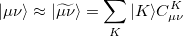$\begin{equation} |\mu \nu \ensuremath{\rangle }\approx |\widetilde{\mu \nu }\ensuremath{\rangle }= \sum _ K |K\ensuremath{\rangle }C_{\mu \nu }^{K} \end{equation}$

(5.19)

Auxiliary basis expansions were introduced long ago, and are now widely recognized as an effective and powerful approach, which is sometimes synonymously called resolution of the identity (RI) or density fitting (DF). When using auxiliary basis expansions, the rate of growth of computational cost of large-scale electronic structure calculations with $n$ is reduced to approximately $n^3$ .

If $n$ is fixed and molecule size increases, auxiliary basis expansions reduce the pre-factor associated with the computation, while not altering the scaling. The important point is that the pre-factor can be reduced by 5 or 10 times or more. Such large speedups are possible because the number of auxiliary functions required to obtain reasonable accuracy, $X$ , has been shown to be only about 3 or 4 times larger than $N$ .

The auxiliary basis expansion coefficients, $\ensuremath{\mathbf{C}}$ , are determined by minimizing the deviation between the fitted distribution and the actual distribution, 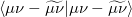$\ensuremath{\langle }\mu \nu -\widetilde{\mu \nu } | {\mu \nu -\widetilde{\mu \nu }} \ensuremath{\rangle }$ , which leads to the following set of linear equations:

$\begin{equation} \sum _ L {\left\langle {K\left| L \right.} \right\rangle } C_{\mu \nu }^ L =\left\langle {K\left| {\mu \nu } \right.} \right\rangle \end{equation}$

(5.20)

Evidently solution of the fit equations requires only two- and three-center integrals, and as a result the (four-center) two-electron integrals can be approximated as the following optimal expression for a given choice of auxiliary basis set:

$\begin{equation} \ensuremath{\langle }\mu \nu |\lambda \sigma \ensuremath{\rangle }\approx \ensuremath{\langle }\widetilde{\mu \nu }|\widetilde{\lambda \sigma }\ensuremath{\rangle }= \sum {K,L}C_{\mu }^{L}\ensuremath{\langle }L|K \ensuremath{\rangle }C_{\lambda \sigma }^ K \end{equation}$

(5.21)

In the limit where the auxiliary basis is complete (i.e. all products of AOs are included), the fitting procedure described above will be exact. However, the auxiliary basis is invariably incomplete (as mentioned above, $X\approx 3N)$ because this is essential for obtaining increased computational efficiency.

Standardized auxiliary basis sets have been developed by the Karlsruhe group for second order perturbation (MP2) calculations [277, 278] of the correlation energy. With these basis sets, small absolute errors (e.g., below 60 $\mu$ Hartree per atom in MP2) and even smaller relative errors in computed energies are found, while the speed-up can be 3–30 fold. This development has made the routine use of auxiliary basis sets for electron correlation calculations possible.

Correlation calculations that can take advantage of auxiliary basis expansions are described in the remainder of this section (MP2, and MP2-like methods) and in Section 5.14 (simplified active space coupled cluster methods such as PP, PP(2), IP, RP). These methods automatically employ auxiliary basis expansions when a valid choice of auxiliary basis set is supplied using the AUX_BASIS keyword which is used in the same way as the BASIS keyword. The PURECART $rem is no longer needed here, even if using a auxiliary basis that does not have a predefined value. There is a built-in automatic procedure that provides the effect of the PURECART $rem in these cases by default.

5.5.1 RI-MP2 Energies and Gradients.

Following common convention, the MP2 energy evaluated approximately using an auxiliary basis is referred to as “resolution of the identity” MP2, or RI-MP2 for short. RI-MP2 energy and gradient calculations are enabled simply by specifying the AUX_BASIS keyword discussed above. As discussed above, RI-MP2 energies [274] and gradients [279, 280] are significantly faster than the best conventional MP2 energies and gradients, and cause negligible loss of accuracy, when an appropriate standardized auxiliary basis set is employed. Therefore they are recommended for jobs where turnaround time is an issue. Disk requirements are very modest; one merely needs to hold various 3-index arrays. Memory requirements grow more slowly than our conventional MP2 algorithms—only quadratically with molecular size. The minimum memory requirement is approximately 3 $X^{2}$ , where $X$ is the number of auxiliary basis functions, for both energy and analytical gradient evaluations, with some additional memory being necessary for integral evaluation and other small arrays.

In fact, for molecules that are not too large (perhaps no more than 20 or 30 heavy atoms) the RI-MP2 treatment of electron correlation is so efficient that the computation is dominated by the initial Hartree-Fock calculation. This is despite the fact that as a function of molecule size, the cost of the RI-MP2 treatment still scales more steeply with molecule size (it is just that the pre-factor is so much smaller with the RI approach). Its scaling remains 5th order with the size of the molecule, which only dominates the initial SCF calculation for larger molecules. Thus, for RI-MP2 energy evaluation on moderate size molecules (particularly in large basis sets), it is desirable to use the dual basis HF method to further improve execution times (see Section 4.8).

5.5.2 Example

Example 5.69 Q-Chem input for an RI-MP2 geometry optimization.

$molecule
   0 1
   O
   H  1  0.9
   F  1  1.4  2  100.
$end

$rem
   JOBTYPE       opt
   METHOD        rimp2
   BASIS         cc-pvtz
   AUX_BASIS     rimp2-cc-pvtz
   SYMMETRY      false
$end

For the size of required memory, the followings need to be considered.

MEM_STATIC

Sets the memory for AO-integral evaluations and their transformations.

TYPE:

INTEGER

DEFAULT:

64

corresponding to 64 Mb.

OPTIONS:

$n$

User-defined number of megabytes.

RECOMMENDATION:

For RI-MP2 calculations, $150(ON + V)$ of MEM_STATIC is required. Because a number of matrices with $N^2$ size also need to be stored, 32–160 Mb of additional MEM_STATIC is needed.

MEM_TOTAL

Sets the total memory available to Q-Chem, in megabytes.

TYPE:

INTEGER

DEFAULT:

2000

2 Gb

OPTIONS:

$n$

User-defined number of megabytes.

RECOMMENDATION:

Use the default, or set to the physical memory of your machine. The minimum requirement is $3X^2$ .

5.5.3 OpenMP Implementation of RI-MP2

An OpenMP RI-MP2 energy algorithm is used by default in Q-Chem 4.1 onward. This can be invoked by using CORR=primp2 for older versions, but note that in 4.01 and below, only RHF/RI-MP2 was supported. Now UHF/RI-MP2 is supported, and the formation of the ‘B’ matrices as well as three center integrals are parallelized. This algorithm uses the remaining memory from the MEM_TOTAL allocation for all computation, which can drastically reduce hard drive reads in the formation of t-amplitudes.

Example 5.70 Example of OpenMP-parallel RI-MP2 job.

$molecule
0 1
 C1
 H1  C1    1.0772600000
 H2  C1    1.0772600000  H1  131.6082400000
$end

$rem
 jobtype                SP
 exchange               HF
 correlation            pRIMP2
 basis                  cc-pVTZ 
 aux_basis              rimp2-cc-pVTZ
 purecart               11111
 symmetry               false
 thresh                 12
 scf_convergence        8
 max_sub_file_num       128
 !time_mp2              true
$end

5.5.4 GPU Implementation of RI-MP2

5.5.4.1 Requirements

Q-Chem currently offers the possibility of accelerating RI-MP2 calculations using graphics processing units (GPUs). Currently, this is implemented for CUDA-enabled NVIDIA graphics cards only, such as (in historical order from 2008) the GeForce, Quadro, Tesla and Fermi cards. More information about CUDA-enabled cards is available at

http://www.nvidia.com/object/cuda_gpus.html

It should be noted that these GPUs have specific power and motherboard requirements.

Software requirements include the installation of the appropriate NVIDIA CUDA driver (at least version 1.0, currently 3.2) and linear algebra library, CUBLAS (at least version 1.0, currently 2.0). These can be downloaded jointly in NVIDIA’s developer website:

http://developer.nvidia.com/object/cuda_3_2_downloads.html

We have implemented a mixed-precision algorithm in order to get better than single precision when users only have single-precision GPUs. This is accomplished by noting that RI-MP2 matrices have a large fraction of numerically “small” elements and a small fraction of numerically “large” ones. The latter can greatly affect the accuracy of the calculation in single-precision only calculations, but calculation involves a relatively small number of compute cycles. So, given a threshold value $\delta$ , we perform a separation between “small” and “large” elements and accelerate the former compute-intensive operations using the GPU (in single-precision) and compute the latter on the CPU (using double-precision). We are thus able to determine how much “double-precision” we desire by tuning the $\delta$ parameter, and tailoring the balance between computational speed and accuracy.

5.5.4.2 Options

CUDA_RI-MP2

Enables GPU implementation of RI-MP2

TYPE:

LOGICAL

DEFAULT:

FALSE

OPTIONS:

FALSE

GPU-enabled MGEMM off

TRUE

GPU-enabled MGEMM on

RECOMMENDATION:

Necessary to set to 1 in order to run GPU-enabled RI-MP2

USECUBLAS_THRESH

Sets threshold of matrix size sent to GPU (smaller size not worth sending to GPU).

TYPE:

INTEGER

DEFAULT:

250

OPTIONS:

n

user-defined threshold

RECOMMENDATION:

Use the default value. Anything less can seriously hinder the GPU acceleration

USE_MGEMM

Use the mixed-precision matrix scheme (MGEMM) if you want to make calculations in your card in single-precision (or if you have a single-precision-only GPU), but leave some parts of the RI-MP2 calculation in double precision)

TYPE:

INTEGER

DEFAULT:

0

OPTIONS:

0

MGEMM disabled

1

MGEMM enabled

RECOMMENDATION:

Use when having single-precision cards

MGEMM_THRESH

Sets MGEMM threshold to determine the separation between “large” and “small” matrix elements. A larger threshold value will result in a value closer to the single-precision result. Note that the desired factor should be multiplied by 10000 to ensure an integer value.

TYPE:

INTEGER

DEFAULT:

10000 (corresponds to 1

OPTIONS:

n

user-defined threshold

RECOMMENDATION:

For small molecules and basis sets up to triple- $\zeta$ , the default value suffices to not deviate too much from the double-precision values. Care should be taken to reduce this number for larger molecules and also larger basis-sets.

5.5.4.3 Input examples

Example 5.71 RI-MP2 double-precision calculation

$comment
RI-MP2 double-precision example
$end
$molecule
0 1
c
h1 c 1.089665
h2 c 1.089665 h1 109.47122063
h3 c 1.089665 h1 109.47122063 h2 120.
h4 c 1.089665 h1 109.47122063 h2 -120.
$end
$rem 
jobtype sp 
exchange hf 
method rimp2 
basis cc-pvdz 
aux_basis rimp2-cc-pvdz 
cuda_rimp2 1
$end

Example 5.72 RI-MP2 calculation with MGEMM

$comment
MGEMM example
$end
$molecule
0 1
c
h1 c 1.089665
h2 c 1.089665 h1 109.47122063
h3 c 1.089665 h1 109.47122063 h2 120.
h4 c 1.089665 h1 109.47122063 h2 -120.
$end
$rem 
jobtype sp 
exchange hf 
method rimp2 
basis cc-pvdz 
aux_basis rimp2-cc-pvdz 
cuda_rimp2 1
USE_MGEMM 1
mgemm_thresh 10000
$end

5.5.5 Spin-biased MP2 (SCS-MP2, SOS-MP2, MOS-MP2, and O2) Energies and Gradients

The accuracy of MP2 calculations can be significantly improved by semi-empirically scaling the opposite-spin (OS) and same-spin (SS) correlation components with separate scaling factors, as shown by Grimme [281]. Scaling with 1.2 and 0.33 (or OS and SS components) defines the SCS-MP2 method, but other parameterizations are desirable for systems involving intermolecular interactions, as in the SCS-MI-MP2 method, which uses 0.40 and 1.29 (for OS and SS components) [282].

Results of similar quality for thermochemistry can be obtained by only retaining and scaling the opposite spin correlation (by 1.3), as was recently demonstrated [283]. Furthermore, the SOS-MP2 energy can be evaluated using the RI approximation together with a Laplace transform technique, in effort that scales only with the 4th power of molecular size. Efficient algorithms for the energy [283] and the analytical gradient [284] of this method are available in Q-Chem 3.0, and offer advantages in speed over MP2 for larger molecules, as well as statistically significant improvements in accuracy.

However, we note that the SOS-MP2 method does systematically underestimate long-range dispersion (for which the appropriate scaling factor is 2 rather than 1.3) but this can be accounted for by making the scaling factor distance-dependent, which is done in the modified opposite spin variant (MOS-MP2) that has recently been proposed and tested [285]. The MOS-MP2 energy and analytical gradient are also available in Q-Chem 3.0 at a cost that is essentially identical with SOS-MP2. Timings show that the 4th-order implementation of SOS-MP2 and MOS-MP2 yields substantial speedups over RI-MP2 for molecules in the 40 heavy atom regime and larger. It is also possible to customize the scale factors for particular applications, such as weak interactions, if required.

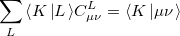
A fourth order scaling SOS-MP2/MOS-MP2 energy calculation can be invoked by setting the CORRELATION keyword to either SOSMP2 or MOSMP2. MOS-MP2 further requires the specification of the $rem variable OMEGA, which tunes the level of attenuation of the MOS operator [285]:

$\begin{equation} g_\omega (r_{12}) = \frac{1}{r_{12} }+c_{\ensuremath{\mathrm{MOS}}} \frac{\ensuremath{\mathrm{erf}}\left( {\omega r_{12} } \right)}{r_{12} } \end{equation}$

(5.22)

The recommended OMEGA value is $\omega = 0.6$ bohr $^{-1}$ [285]. The fast algorithm makes use of auxiliary basis expansions and therefore, the keyword AUX_BASIS should be set consistently with the user’s choice of BASIS. Fourth-order scaling analytical gradient for both SOS-MP2 and MOS-MP2 are also available and is automatically invoked when JOBTYPE is set to OPT or FORCE. The minimum memory requirement is 3 $X^{2}$ , where $X$ = the number of auxiliary basis functions, for both energy and analytical gradient evaluations. Disk space requirement for closed shell calculations is $\sim 2OVX$ for energy evaluation and $\sim 4OVX$ for analytical gradient evaluation.

More recently, Brueckner orbitals (BO) are introduced into SOSMP2 and MOSMP2 methods to resolve the problems of symmetry breaking and spin contamination that are often associated with Hartree-Fock orbitals. So the molecular orbitals are optimized with the mean-field energy plus a correlation energy taken as the opposite-spin component of the second-order many-body correlation energy, scaled by an empirically chosen parameter. This “optimized second-order opposite-spin” abbreviated as O2 method [286] requires fourth-order computation on each orbital iteration. O2 is shown to yield predictions of structure and frequencies for closed-shell molecules that are very similar to scaled MP2 methods. However, it yields substantial improvements for open-shell molecules, where problems with spin contamination and symmetry breaking are shown to be greatly reduced.

Summary of key $rem variables to be specified:

CORRELATION	RIMP2
	SOSMP2
	MOSMP2
JOBTYPE	sp (default) single point energy evaluation
	opt geometry optimization with analytical gradient
	force force evaluation with analytical gradient
BASIS	user’s choice (standard or user-defined: GENERAL or MIXED)
AUX_BASIS	corresponding auxiliary basis (standard or user-defined:
	AUX_GENERAL or AUX_MIXED
OMEGA	no default $n$ ; use $\omega = n/1000$ . The recommended value is
	$n=600$ ( $\omega = 0.6$ bohr $^{-1}$ )
N_FROZEN_CORE	Optional
N_FROZEN_VIRTUAL	Optional
SCS	Turns on spin-component scaling with SCS-MP2(1),
	SOS-MP2(2), and arbitrary SCS-MP2(3)

5.5.6 Examples

Example 5.73 Example of SCS-MP2 geometry optimization

$molecule
0 1
C
H  1 1.0986
H  1 1.0986 2 109.5
H  1 1.0986 2 109.5 3 120.0 0
H  1 1.0986 2 109.5 3 -120.0 0
$end

$rem
jobtype           opt
exchange          hf
correlation       rimp2
basis             aug-cc-pvdz
aux_basis         rimp2-aug-cc-pvdz
basis2            racc-pvdz            Optional Secondary basis
thresh            12
scf_convergence   8
max_sub_file_num  128
SCS               1                    Turn on spin-component scaling
dual_basis_energy true                 Optional dual-basis approximation
n_frozen_core     fc       
symmetry          false                
sym_ignore        true
$end

Example 5.74 Example of SCS-MI-MP2 energy calculation

$molecule
0 1
C       0.000000        -0.000140       1.859161
H       -0.888551       0.513060        1.494685
H       0.888551        0.513060        1.494685
H       0.000000        -1.026339       1.494868
H       0.000000        0.000089        2.948284
C       0.000000        0.000140        -1.859161
H       0.000000        -0.000089       -2.948284
H       -0.888551       -0.513060       -1.494685
H       0.888551        -0.513060       -1.494685
H       0.000000        1.026339        -1.494868
$end

$rem
jobtype           sp
exchange          hf
correlation       rimp2
basis             aug-cc-pvtz
aux_basis         rimp2-aug-cc-pvtz
basis2            racc-pvtz            Optional Secondary basis
thresh            12
scf_convergence   8
max_sub_file_num  128
SCS               3                    Spin-component scale arbitrarily
SOS_FACTOR        0400000              Specify OS parameter
SSS_FACTOR        1290000              Specfiy SS parameter
dual_basis_energy true                 Optional dual-basis approximation
n_frozen_core     fc       
symmetry          false                
sym_ignore        true
$end

Example 5.75 Example of SOS-MP2 geometry optimization

$molecule
   0 3
   C1
   H1   C1   1.07726
   H2   C1   1.07726   H1  131.60824
$end

$rem
   JOBTYPE        opt
   METHOD         sosmp2
   BASIS          cc-pvdz
   AUX_BASIS      rimp2-cc-pvdz
   UNRESTRICTED   true
   SYMMETRY       false
$end

Example 5.76 Example of MOS-MP2 energy evaluation with frozen core approximation

$molecule
   0 1
   Cl 
   Cl 1 2.05
$end

$rem
   JOBTYPE           sp
   METHOD            mosmp2
   OMEGA             600 
   BASIS             cc-pVTZ
   AUX_BASIS         rimp2-cc-pVTZ
   N_FROZEN_CORE     fc
   THRESH            12
   SCF_CONVERGENCE   8
$end

Example 5.77 Example of O2 methodology applied to $\mbox{${\cal {O}}({N^4})$}$ SOSMP2

   $molecule
   1 2
   F
   H 1 1.001
$end

$rem
   UNRESTRICTED      TRUE
   JOBTYPE           FORCE            Options are SP/FORCE/OPT
   EXCHANGE          HF
   DO_O2             1                O2 with O(N^4) SOS-MP2 algorithm
   SOS_FACTOR        1000000          Opposite Spin scaling factor = 1.0
   SCF_ALGORITHM     DIIS_GDM
   SCF_GUESS         GWH
   BASIS             sto-3g
   AUX_BASIS         rimp2-vdz
   SCF_CONVERGENCE   8
   THRESH            14
   SYMMETRY          FALSE
   PURECART          1111
$end

Example 5.78 Example of O2 methodology applied to $\mbox{${\cal {O}}({N^4})$}$ MOSMP2

$molecule
   1 2
   F
   H 1 1.001
$end

$rem
   UNRESTRICTED      TRUE
   JOBTYPE           FORCE            Options are SP/FORCE/OPT
   EXCHANGE          HF
   DO_O2             2                O2 with O(N^4) MOS-MP2 algorithm
   OMEGA             600              Omega = 600/1000 = 0.6 a.u.
   SCF_ALGORITHM     DIIS_GDM
   SCF_GUESS         GWH
   BASIS             sto-3g
   AUX_BASIS         rimp2-vdz
   SCF_CONVERGENCE   8
   THRESH            14
   SYMMETRY          FALSE
   PURECART          1111
$end

5.5.7 RI-TRIM MP2 Energies

The triatomics in molecules (TRIM) local correlation approximation to MP2 theory [269] was described in detail in Section 5.4.1 which also discussed our implementation of this approach based on conventional four-center two-electron integrals. Q-Chem 3.0 also includes an auxiliary basis implementation of the TRIM model. The new RI-TRIM MP2 energy algorithm [287] greatly accelerates these local correlation calculations (often by an order of magnitude or more for the correlation part), which scale with the 4th power of molecule size. The electron correlation part of the calculation is speeded up over normal RI-MP2 by a factor proportional to the number of atoms in the molecule. For a hexadecapeptide, for instance, the speedup is approximately a factor of 4 [287]. The TRIM model can also be applied to the scaled opposite spin models discussed above. As for the other RI-based models discussed in this section, we recommend using RI-TRIM MP2 instead of the conventional TRIM MP2 code whenever run-time of the job is a significant issue. As for RI-MP2 itself, TRIM MP2 is invoked by adding AUX_BASIS $rems to the input deck, in addition to requesting CORRELATION = RILMP2.

Example 5.79 Example of RI-TRIM MP2 energy evaluation

$molecule
   0 3
   C1
   H1   C1   1.07726
   H2   C1   1.07726   H1   131.60824
$end

$rem
   METHOD         rilmp2 
   BASIS          cc-pVDZ
   AUX_BASIS      rimp2-cc-pVDZ
   PURECART       1111
   UNRESTRICTED   true
   SYMMETRY       false
$end

5.5.8 Dual-Basis MP2

The successful computational cost speedups of the previous sections often leave the cost of the underlying SCF calculation dominant. The dual-basis method provides a means of accelerating the SCF by roughly an order of magnitude, with minimal associated error (see Section 4.8). This dual-basis reference energy may be combined with RI-MP2 calculations for both energies [233, 237] and analytic first derivatives [235]. In the latter case, further savings (beyond the SCF alone) are demonstrated in the gradient due to the ability to solve the response ( $Z$ -vector) equations in the smaller basis set. Refer to Section 4.8 for details and job control options.