4.4 Density Functional Theory
4.4.1 Introduction
DFT [20, 21, 22, 23] has emerged as an accurate, alternative first-principles approach to quantum mechanical molecular investigations. DFT calculations account for the overwhelming majority of all quantum chemistry calculations, not only because of its proven chemical accuracy, but also because of its relatively low computational expense, comparable to Hartree-Fock theory but with treatment of electron correlation that is neglected in a HF calculation. These two features suggest that DFT is likely to remain a leading method in the quantum chemist’s toolkit well into the future. Q-Chem contains fast, efficient and accurate algorithms for all popular density functionals, making calculations on large molecules possible and practical.
DFT is primarily a theory of electronic ground state structures based on the electron density,  , as opposed to the many-electron wave function,
  . (It’s excited-state extension, time-dependent DFT, is discussed in Section 6.3.) There are a number of distinct similarities and differences between traditional wave function approaches and modern DFT methodologies. First, the essential building blocks of the many-electron wave function
  are single-electron orbitals, which are directly analogous to the Kohn-Sham orbitals in the DFT framework. Second, both the electron density and the many-electron wave function tend to be constructed via a SCF approach that requires the construction of matrix elements that are conveniently very similar.
However, traditional ab initio approaches using the many-electron wave function as a foundation must resort to a post-SCF calculation (Chapter 5) to incorporate correlation effects, whereas DFT approaches incorporate correlation at the SCF level. Post-SCF methods, such as perturbation theory or coupled-cluster theory are extremely expensive relative to the SCF procedure. On the other hand, while the DFT approach is exact in principle, in practice it relies on modeling an unknown exchange-correlation energy functional. While more accurate forms of such functionals are constantly being developed, there is no systematic way to improve the functional to achieve an arbitrary level of accuracy. Thus, the traditional approaches offer the possibility of achieving a systematically-improvable level of accuracy, but can be computationally demanding, whereas DFT approaches offer a practical route, but the theory is currently incomplete.
4.4.2 Kohn-Sham Density Functional Theory
The density functional theory by Hohenberg, Kohn, and Sham [24, 25] stems from the original work of Dirac [26], who found that the exchange energy of a uniform electron gas may be calculated exactly, knowing only the charge density. However, while the more traditional DFT constitutes a direct approach where the necessary equations contain only the electron density, difficulties associated with the kinetic energy functional obstructed the extension of DFT to anything more than a crude level of approximation. Kohn and Sham developed an indirect approach to the kinetic energy functional, which transformed DFT into a practical tool for quantum-chemical calculations.
Within the Kohn-Sham formalism [25], the ground state electronic energy,  , can be written as
 |
(4.34) |
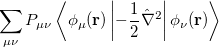
where  is the kinetic energy,
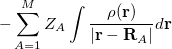
  is the electron–nuclear interaction energy,
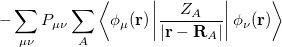
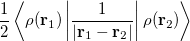
  is the Coulomb self-interaction of the electron density, and
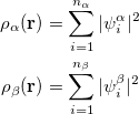
  is the exchange-correlation energy. Adopting an unrestricted format, the
  and
and  total electron densities can be written as
 |
(4.35) |
where  and
and  are the number of alpha and beta electron respectively, and
  are the Kohn-Sham orbitals. Thus, the total electron density is
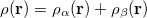
 |
(4.38) |
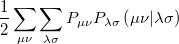
Within a finite basis set [27], the density is represented by
 |
(4.39) |
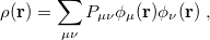
where the  are the elements of the one-electron density matrix; see Eq. eq:P(mu,nu) in the discussion of Hartree-Fock theory. The various energy components in Eq. eq:DFT_energy_components can now be written
 |
 |
 |
|||
 |
|
 |
(4.40) | ||
 |
|
 |
|||
|
|
 |
(4.41) | ||
 |
|
 |
|||
|
|
 |
(4.42) | ||
 |
|
![$\displaystyle \int f\left[\rho (\ensuremath{\mathbf{r}}),\hat\nabla \rho (\ensuremath{\mathbf{r}}),\ldots \right] d\ensuremath{\mathbf{r}} \label{E_ XC} $](images/img-0128.png) |
(4.43) |
Minimizing with respect to the unknown Kohn-Sham orbital coefficients yields a set of matrix equations exactly analogous to Pople-Nesbet equations of the UHF case, Eq. eq:Pople-Nesbet, but with modified Fock matrix elements [cf. Eq. eq:F(mu,nu)]
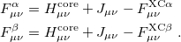 |
(4.44) |
Here,  and
and  are the exchange-correlation parts of the Fock matrices and depend on the exchange-correlation functional used. UHF theory is recovered as a special case simply by taking
  , and similarly for . Thus, the density and energy are obtained in a manner analogous to that for the HF method. Initial guesses are made for the MO coefficients and an iterative process is applied until self-consistency is achieved.
4.4.3 Overview of Available Functionals
Q-Chem currently has more than 25 exchange functionals as well as more than 25 correlation functionals, and in addition over 100 exchange-correlation (xc) functionals, which refer to functionals that are not separated into exchange and correlation parts, either because the way in which they were parameterized renders such a separation meaningless (e.g., B97-D[28] or  B97X[29]) or else they are a standard linear combination of exchange and correlation (e.g., PBE[30] or B3LYP[31]). User-defined xc functionals can be created as specified linear combinations of any of the 25+ exchange functionals and/or the 25+ correlation functionals.
KS-DFT functionals can be organized onto a ladder with five rungs, in a classification scheme (“Jacob’s Ladder”) proposed by John Perdew[32] in 2001. The first rung contains a functional that only depends on the (spin-)density  , namely, the local spin-density approximation (LSDA). This functionals is exact for the infinite uniform electron gas (UEG), but are highly inaccurate for molecular properties whose densities exhibit significant inhomogeneity. To improve upon the weaknesses of the LSDA, it is necessary to introduce an ingredient that can account for inhomogeneities in the density: the density gradient,
  . These generalized gradient approximation (GGA) functionals define the second rung of Jacob’s Ladder and tend to improve significantly upon the LSDA. Two additional ingredients that can be used to further improve the performance of GGA functionals are either the Laplacian of the density
  , and/or the kinetic energy density,
 |
(4.47) |
While functionals that employ both of these options are available in Q-Chem, the kinetic energy density is by far the more popular ingredient and has been used in many modern functionals to add flexibility to the functional form with respect to both constraint satisfaction (non-empirical functionals) and least-squares fitting (semi-empirical parameterization). Functionals that depend on either of these two ingredients belong to the third rung of the Jacob’s Ladder and are called meta-GGAs. These meta-GGAs often further improve upon GGAs in areas such as thermochemistry, kinetics (reaction barrier heights), and even non-covalent interactions.
Functionals on the fourth rung of Jacob’s Ladder are called hybrid density functionals. This rung contains arguably the most popular density functional of our time, B3LYP, the first functional to see widespread application in chemistry. “Global” hybrid (GH) functionals such as B3LYP (as distinguished from the “range-separated hybrids" introduced below) add a constant fraction of “exact” (Hartree-Fock) exchange to any of functionals from the first three rungs. Thus, hybrid LSDA, hybrid GGA, and hybrid meta-GGA functionals can be constructed, although the latter two types are much more common. As an example, the formula for the B3LYP functional, as implemented in Q-Chem, is
 |
(4.48) |
where  ,
,  , and
, and  .
.
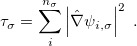
A more recent approach to introducing exact exchange into the functional form is via range separation. Range-separated hybrid (RSH) functionals split the exact exchange contribution into a short-range (SR) component and a long-range (LR) component, often by means of the error function (erf) and complementary error function ( ):
):
 |
(4.49) |
The first term on the right in Eq. () is singular but short-range, and decays to zero on a length scale of  , while the second term constitutes a non-singular, long-range background. An RSH xc functional can be expressed generically as
 |
(4.50) |
where the SR and LR parts of the Coulomb operator are used, respectively, to evaluate the HF exchange energies  and
and  . The corresponding DFT exchange functional is partitioned in the same manner, but the correlation energy
  is evaluated using the full Coulomb operator,
  . Of the two linear parameters in Eq. eq:RSHGGA,
  is usually either set to 1 to define long-range corrected (LRC) RSH functionals (see Section 4.4.6) or else set to 0, which defines screened-exchange (SE) RSH functionals. On the other hand, the fraction of short-range exact exchange (
 ) can either be determined via least-squares fitting, theoretically justified using the adiabatic connection, or simply set to zero. As with the global hybrids, RSH functionals can be fashioned using all of the ingredients from the lower three rungs. The rate at which the local DFT exchange is turned off and the non-local exact exchange is turned on is controlled by the parameter . Large values of tend to lead to attenuators that are less smooth (unless the fraction of short-range exact exchange is very large), while small values of (e.g.,
  0.2–0.3 bohr
 ) are the most common in semi-empirical RSH functionals.
The final rung on Jacob’s Ladder contains functionals that utilize not only occupied orbitals (via exact exchange), but virtual orbitals as well (via methods such as MP2 or RPA). These double hybrids (DH) are the most expensive density functionals available in Q-Chem, but can also be very accurate. The most basic form of a DH functional is
 |
(4.51) |
As with hybrids, the coefficients can either be theoretically motivated or empirically determined. In addition, double hybrids can utilize exact exchange both globally or via range-separation, and their components can be as primitive as LSDA or as advanced as in meta-GGA functionals. More information on double hybrids can be found in Section 4.4.8.
Finally, the last major advance in KS-DFT in recent years has been the development of methods that are capable of accurately describing non-covalent interactions, particularly dispersion. All of the functionals from Jacob’s Ladder can technically be combined with these dispersion corrections, although in some cases the combination is detrimental, particularly for semi-empirical functionals that were parameterized in part using data sets of non-covalent interactions, and already tend to overestimate non-covalent interaction energies. The most popular such methods available in Q-Chem are the:
Non-local correlation (NLC) functionals (Section 4.4.7.1), including those of Vydrov and Van Voorhis[33, 34] (VV09 and VV10) and of Lundqvist and Langreth[35, 36] (vdW-DF-04 and vdW-DF-10).
Damped, atom–atom pairwise empirical dispersion potentials from Grimme[28, 37, 38] [DFT-D2, DFT-CHG, and DFT-D3(0)]; see Section 4.4.7.2.
The exchange-dipole models (XDM) of Johnson and Becke (XDM6 and XDM10); see Section 4.4.7.3.
Below, we categorize the functionals that are available in Q-Chem, including exchange functionals (Section 4.4.3.1), correlation functionals (Section 4.4.3.2), and exchange-correlation functionals (Section 4.4.3.3). Within each category the functionals will be categorized according to Jacob’s Ladder. Exchange and correlation functionals can be invoked using the $rem variables EXCHANGE and CORRELATION, while the exchange-correlation functionals can be invoked either by setting the $rem variable METHOD or alternatively (in most cases, and for backwards compatibility with earlier versions of Q-Chem) by using $rem variable EXCHANGE. Some caution is warranted here. While setting METHOD to PBE, for example, requests the Perdew-Burke-Ernzerhof (PBE) exchange-correlation functional,[30] which includes both PBE exchange and PBE correlation, setting EXCHANGE = PBE requests only the exchange component and setting CORRELATION = PBE requests only the correlation component. Setting both of these values is equivalent to specifying METHOD = PBE.
Single-Point |
Optimization |
Frequency |
|
Ground State |
LSDA |
LSDA |
LSDA |
GGA |
GGA |
GGA |
|
meta-GGA |
meta-GGA |
— |
|
GH |
GH |
GH |
|
RSH |
RSH |
RSH |
|
NLC |
NLC |
— |
|
DFT-D |
DFT-D |
DFT-D |
|
XDM |
— |
— |
|
TDDFT |
LSDA |
LSDA |
LSDA |
GGA |
GGA |
GGA |
|
meta-GGA |
— |
— |
|
GH |
GH |
GH |
|
RSH |
RSH |
— |
|
— |
— |
— |
|
DFT-D |
DFT-D |
DFT-D |
|
— |
— |
— |
|
|
|||
|
|||


 OpenMP parallelization available
 MPI parallelization available
Finally, Table 4.2 provides a summary, arranged according to Jacob’s Ladder, of which categories of functionals are available with analytic first derivatives (for geometry optimizations) or second derivatives (for vibrational frequency calculations); if analytic derivatives are not available for the requested job type, Q-Chem will automatically generate them via finite-difference. Also listed in Table 4.2 are which functionals are avaiable for excited-state time-dependent DFT (TDDFT) calculations, as described in Section 6.3. Lastly, Table 4.2 describes which functionals have been parallelized with OpenMP and/or MPI.
4.4.3.1 Exchange Functionals
Note: All exchange functionals in this section can be invoked using the $rem variable EXCHANGE. Popular and/or recommended functionals within each class are listed first and indicated in bold. The rest are in alphabetical order.
Local Spin-Density Approximation (LSDA)
Slater – Slater-Dirac exchange functional (X
method with  )[26]
)[26] SR_LSDA (BNL) – Short-range version of the Slater-Dirac exchange functional[39]
Generalized Gradient Approximation (GGA)
PBE – Perdew, Burke, and Ernzerhof exchange functional[30]
B88 – Becke exchange functional from 1988[40]
revPBE – Zhang and Yang one-parameter modification of the PBE exchange functional[41]
AK13 – Armiento-Kümmel exchange functional from 2013[42]
B86 – Becke exchange functional (X
 ) from 1986[43]
 G96 – Gill exchange functional from 1996[44]
mB86 – Becke “modified gradient correction” exchange functional from 1986[45]
mPW91 – modified version (Adamo and Barone) of the 1991 Perdew-Wang exchange functional[46]
muB88 (
 B88) – Short-range version of the B88 exchange functional by Hirao and coworkers[47]
 muPBE (
PBE) – Short-range version of the PBE exchange functional by Hirao and coworkers[47] OPTX – Two-parameter exchange functional by Handy and Cohen[48]
PBEsol – PBE exchange functional modified for solids[49]
PW86 – Perdew-Wang exchange functional from 1986[50]
PW91 – Perdew-Wang exchange functional from 1991[51]
RPBE – Hammer, Hansen, and Norskov exchange functional (modification of PBE)[52]
rPW86 – revised version (Murray et al.) of the 1986 Perdew-Wang exchange functional[53]
SOGGA – Second-order GGA functional by Zhao and Truhlar[54]
wPBE (
PBE) – Henderson et al. model for the PBE GGA short-range exchange hole[55]
Meta-Generalized Gradient Approximation (meta-GGA)
TPSS – Tao, Perdew, Staroverov, and Scuseria exchange functional[56]
revTPSS – Revised version of the TPSS exchange functional[57]
modTPSS – One-parameter version of the TPSS exchange functional[58]
PKZB – Perdew, Kurth, Zupan, and Blaha exchange functional[59]
regTPSS – Regularized (fixed order of limits issue) version of the TPSS exchange functional[60]
SCAN – Strongly Constrained and Appropriately Normed exchange functional[61]
4.4.3.2 Correlation Functionals
Note: All correlation functionals in this section can be invoked using the $rem variable CORRELATION. Popular and/or recommended functionals within each class are listed first and indicated in bold. The rest are in alphabetical order.
Local Spin-Density Approximation (LSDA)
PW92 – Perdew-Wang parameterization of the LSDA correlation energy from 1992[62]
VWN5 (VWN) – Vosko-Wilk-Nusair parameterization of the LSDA correlation energy #5[63]
Liu-Parr – Liu-Parr
 model from the functional expansion formulation[64]
 PK09 – Proynov-Kong parameterization of the LSDA correlation energy from 2009[65]
PW92RPA – Perdew-Wang parameterization of the LSDA correlation energy from 1992 with RPA values[62]
PZ81 – Perdew-Zunger parameterization of the LSDA correlation energy from 1981[66]
VWN1 – Vosko-Wilk-Nusair parameterization of the LSDA correlation energy #1[63]
VWN1RPA – Vosko-Wilk-Nusair parameterization of the LSDA correlation energy #1 with RPA values[63]
VWN2 – Vosko-Wilk-Nusair parameterization of the LSDA correlation energy #2[63]
VWN3 – Vosko-Wilk-Nusair parameterization of the LSDA correlation energy #3[63]
VWN4 – Vosko-Wilk-Nusair parameterization of the LSDA correlation energy #4[63]
Wigner – Wigner correlation functional (simplification of LYP)[67, 68]
Generalized Gradient Approximation (GGA)
PBE – Perdew, Burke, and Ernzerhof correlation functional[30]
LYP – Lee-Yang-Parr opposite-spin correlation functional[69]
P86 – Perdew-Wang correlation functional from 1986 based on the PZ81 LSDA functional[70]
P86VWN5 – Perdew-Wang correlation functional from 1986 based on the VWN5 LSDA functional[70]
PBEsol – PBE correlation functional modified for solids[49]
PW91 – Perdew-Wang correlation functional from 1991[51]
regTPSS – Slight modification of the PBE correlation functional (also called vPBEc)[60]
Meta-Generalized Gradient Approximation (meta-GGA)
TPSS – Tao, Perdew, Staroverov, and Scuseria correlation functional[56]
revTPSS – Revised version of the TPSS correlation functional[57]
B95 – Becke’s two-parameter correlation functional from 1995[71]
PK06 – Proynov-Kong “tLap” functional with
 and Laplacian dependence[72]
 PKZB – Perdew, Kurth, Zupan, and Blaha correlation functional[59]
SCAN – Strongly Constrained and Appropriately Normed correlation functional[61]
4.4.3.3 Exchange-Correlation Functionals
Note: All exchange-correlation functionals in this section can be invoked using the $rem variable METHOD. For backwards compatibility, all of the exchange-correlation functionals except for the ones marked with an asterisk can be utilized with the $rem variable EXCHANGE. Popular and/or recommended functionals within each class are listed first and indicated in bold. The rest are in alphabetical order.
Local Spin-Density Approximation (LSDA)
LDA* – Slater LSDA exchange + VWN5 LSDA correlation
Generalized Gradient Approximation (GGA)
B97-D3(0) – B97-D with a fitted DFT-D3(0) tail instead of the original DFT-D2 tail[38]
B97-D – 9-parameter dispersion-corrected (DFT-D2) functional by Grimme[28]
VV10 – rPW86 GGA exchange + PBE GGA correlation + VV10 non-local correlation[34]
PBE* – PBE GGA exchange + PBE GGA correlation
BLYP* – B88 GGA exchange + LYP GGA correlation
revPBE* – revPBE GGA exchange + PBE GGA correlation
BOP – B88 GGA exchange + BOP “one-parameter progressive” GGA correlation[73]
BP86* – B88 GGA exchange + P86 GGA correlation
BP86VWN* – B88 GGA exchange + P86VWN5 GGA correlation
EDF1 – Modification of BLYP to give good performance in the 6-31+G* basis set[74]
EDF2 – Modification of B3LYP to give good performance in the cc-pVTZ basis set for frequencies[75]
GAM – 21-parameter nonseparable gradient approximation functional by Truhlar and coworkers[76]
HCTH120 (HCTH/120) – 15-parameter functional trained on 120 systems by Boese et al.[77]
HCTH147 (HCTH/147) – 15-parameter functional trained on 147 systems by Boese et al.[77]
HCTH407 (HCTH/407) – 15-parameter functional trained on 407 systems by Boese and Handy[78]
HCTH93 (HCTH/93) – 15-parameter functional trained on 93 systems by Handy and coworkers[79]
N12 – 21-parameter nonseparable gradient approximation functional by Peverati and Truhlar[80]
PBEOP – PBE GGA exchange + PBEOP “one-parameter progressive” GGA correlation[73]
PBEsol* – PBEsol GGA exchange + PBEsol GGA correlation
PW91* – PW91 GGA exchange + PW91 GGA correlation
SOGGA* – SOGGA GGA exchange + PBE GGA correlation
SOGGA11 – 20-parameter functional by Peverati, Zhao, and Truhlar[81]
Meta-Generalized Gradient Approximation (meta-GGA)
B97M-V – 12-parameter combinatorially-optimized, dispersion-corrected (VV10) functional by Mardirossian and Head-Gordon[82]
M06-L – 34-parameter functional by Zhao and Truhlar[83]
TPSS* – TPSS meta-GGA exchange + TPSS meta-GGA correlation
revTPSS* – revTPSS meta-GGA exchange + revTPSS meta-GGA correlation
M11-L – 44-parameter dual-range functional by Peverati and Truhlar[84]
MGGA_MS0 – MGGA_MS0 meta-GGA exchange + regTPSS GGA correlation[85]
MGGA_MS1 – MGGA_MS1 meta-GGA exchange + regTPSS GGA correlation[86]
MGGA_MS2 – MGGA_MS2 meta-GGA exchange + regTPSS GGA correlation[86]
MGGA_MVS – MGGA_MVS meta-GGA exchange + regTPSS GGA correlation[87]
MN12-L – 58-parameter meta-nonseparable gradient approximation functional by Peverati and Truhlar[88]
MN15-L – 58-parameter meta-nonseparable gradient approximation functional by Yu, He, and Truhlar[89]
PKZB* – PKZB meta-GGA exchange + PKZB meta-GGA correlation
SCAN* – SCAN meta-GGA exchange + SCAN meta-GGA correlation
t-HCTH (
-HCTH) – 16-parameter functional by Boese and Handy[90] VSXC – 21-parameter functional by Voorhis and Scuseria[91]
Global Hybrid Generalized Gradient Approximation (GH GGA)
B3LYP – 20% HF exchange + 8% Slater LSDA exchange + 72% B88 GGA exchange + 19% VWN1RPA LSDA correlation + 81% LYP GGA correlation[31]
PBE0 – 25% HF exchange + 75% PBE GGA exchange + PBE GGA correlation[92]
revPBE0 – 25% HF exchange + 75% revPBE GGA exchange + PBE GGA correlation
B97 – Becke’s original 10-parameter density functional with 19.43% HF exchange[93]
B1LYP – 25% HF exchange + 75% B88 GGA exchange + LYP GGA correlation
B1PW91 – 25% HF exchange + 75% B88 GGA exchange + PW91 GGA correlation
B3LYP5 – 20% HF exchange + 8% Slater LSDA exchange + 72% B88 GGA exchange + 19% VWN5 LSDA correlation + 81% LYP GGA correlation
B3P86 – 20% HF exchange + 8% Slater LSDA exchange + 72% B88 GGA exchange+ 19% VWN1RPA LSDA correlation + 81% P86 GGA correlation
B3PW91 – 20% HF exchange + 8% Slater LSDA exchange + 72% B88 GGA exchange+ 19% PW92 LSDA correlation + 81% PW91 GGA correlation
B5050LYP – 50% HF exchange + 8% Slater LSDA exchange + 42% B88 GGA exchange + 19% VWN5 LSDA correlation + 81% LYP GGA correlation[94]
B97-1 – Self-consistent parameterization of Becke’s B97 density functional with 21% HF exchange[79]
B97-2 – Re-parameterization of B97 by Tozer and coworkers with 21% HF exchange[95]
B97-3 – 16-parameter version of B97 by Keal and Tozer with
 26.93% HF exchange[96]
 B97-K – Re-parameterization of B97 for kinetics by Boese and Martin with 42% HF exchange[97]
BHHLYP – 50% HF exchange + 50% B88 GGA exchange + LYP GGA correlation
MPW1K – 42.8% HF exchange + 57.2% mPW91 GGA exchange + PW91 GGA correlation[98]
MPW1LYP – 25% HF exchange + 75% mPW91 GGA exchange + LYP GGA correlation
MPW1PBE – 25% HF exchange + 75% mPW91 GGA exchange + PBE GGA correlation
MPW1PW91 – 25% HF exchange + 75% mPW91 GGA exchange + PW91 GGA correlation
O3LYP – 11.61% HF exchange +
7.1% Slater LSDA exchange + 81.33% OPTX GGA exchange + 19% VWN5 LSDA correlation + 81% LYP GGA correlation[99] PBE50 – 50% HF exchange + 50% PBE GGA exchange + PBE GGA correlation
SOGGA11-X – 21-parameter functional with 40.15% HF exchange by Peverati and Truhlar[100]
X3LYP – 21.8% HF exchange + 7.3% Slater LSDA exchange +
54.24% B88 GGA exchange + 16.66% PW91 GGA exchange + 12.9% VWN1RPA LSDA correlation + 87.1% LYP GGA correlation[101]
Global Hybrid Meta-Generalized Gradient Approximation (GH meta-GGA)
M06-2X – 29-parameter functional with 54% HF exchange by Zhao and Truhlar[102]
M08-HX – 47-parameter functional with 52.23% HF exchange by Zhao and Truhlar[103]
TPSSh – 10% HF exchange + 90% TPSS meta-GGA exchange + TPSS meta-GGA correlation[104]
revTPSSh – 10% HF exchange + 90% revTPSS meta-GGA exchange + revTPSS meta-GGA correlation[105]
B1B95 – 28% HF exchange + 72% B88 GGA exchange + B95 meta-GGA correlation[71]
B3TLAP – 17.13% HF exchange + 9.66% Slater LSDA exchange + 72.6% B88 GGA exchange + PK06 meta-GGA correlation[72, 106]
BB1K – 42% HF exchange + 58% B88 GGA exchange + B95 meta-GGA correlation[107]
BMK – Boese-Martin functional for kinetics with 42% HF exchange[97]
dlDF – Dispersionless density functional (based on the M05-2X functional form) by Szalewicz and coworkers[108]
M05 – 22-parameter functional with 28% HF exchange by Zhao, Schultz, and Truhlar[109]
M05-2X – 19-parameter functional with 56% HF exchange by Zhao, Schultz, and Truhlar[110]
M06 – 33-parameter functional with 27% HF exchange by Zhao and Truhlar[102]
M06-HF – 32-parameter functional with 100% HF exchange by Zhao and Truhlar[111]
M08-SO – 44-parameter functional with 56.79% HF exchange by Zhao and Truhlar[103]
MGGA_MS2h – 9% HF exchange + 91 % MGGA_MS2 meta-GGA exchange + regTPSS GGA correlation[86]
MGGA_MVSh – 25% HF exchange + 75 % MGGA_MVS meta-GGA exchange + regTPSS GGA correlation[87]
MPW1B95 – 31% HF exchange + 69% mPW91 GGA exchange + B95 meta-GGA correlation[112]
MPWB1K – 44% HF exchange + 56% mPW91 GGA exchange + B95 meta-GGA correlation[112]
PW6B95 – 6-parameter combination of 28 % HF exchange, 72 % optimized PW91 GGA exchange, and re-optimized B95 meta-GGA correlation by Zhao and Truhlar[113]
PWB6K – 6-parameter combination of 46 % HF exchange, 54 % optimized PW91 GGA exchange, and re-optimized B95 meta-GGA correlation by Zhao and Truhlar[113]
SCAN0 – 25% HF exchange + 75% SCAN meta-GGA exchange + SCAN meta-GGA correlation[114]
t-HCTHh (
-HCTHh) – 17-parameter functional with 15% HF exchange by Boese and Handy[90]
Range-Separated Hybrid Generalized Gradient Approximation (RSH GGA)
wB97X-V (
B97X-V) – 10-parameter combinatorially-optimized, dispersion-corrected (VV10) functional with 16.7% SR HF exchange, 100% LR HF exchange, and  [115]
[115] wB97X-D3 (
B97X-D3) – 16-parameter dispersion-corrected (DFT-D3(0)) functional with 19.57% SR HF exchange, 100% LR HF exchange, and  [116]
[116] wB97X-D (
B97X-D) – 15-parameter dispersion-corrected (DFT-CHG) functional with 22.2% SR HF exchange, 100% LR HF exchange, and  [37]
[37] LC-VV10 – 0% SR HF exchange + 100% LR HF exchange +
PBE GGA exchange + PBE GGA correlation + VV10 non-local correlation (=0.45)[34] CAM-B3LYP – Coulomb-attenuating method functional by Handy and coworkers[117]
LRC-BOP (LRC-
BOP)– 0% SR HF exchange + 100% LR HF exchange + muB88 GGA exchange + BOP GGA correlation (=0.47)[118] LRC-wPBE (LRC-
PBE) – 0% SR HF exchange + 100% LR HF exchange + PBE GGA exchange + PBE GGA correlation (=0.3)[119] LRC-wPBEh (LRC-
PBEh) – 20% SR HF exchange + 100% LR HF exchange + 80% PBE GGA exchange + PBE GGA correlation (=0.2)[120] N12-SX – 26-parameter non-separable GGA with 25% SR HF exchange, 0% LR HF exchange, and
 [121]
[121] wB97 (
B97) – 13-parameter functional with 0% SR HF exchange, 100% LR HF exchange, and  [29]
[29] wB97X (
B97X) – 14-parameter functional with 15.77% SR HF exchange, 100% LR HF exchange, and [29]
Range-Separated Hybrid Meta-Generalized Gradient Approximation (RSH meta-GGA)
wB97M-V (
B97M-V) – 12-parameter combinatorially-optimized, dispersion-corrected (VV10) functional with 15% SR HF exchange, 100% LR HF exchange, and [82] M11 – 40-parameter functional with 42.8% SR HF exchange, 100% LR HF exchange, and
[122] MN12-SX – 58-parameter non-separable meta-GGA with 25% SR HF exchange, 0% LR HF exchange, and
[121] wM05-D (
M05-D) – 21-parameter dispersion-corrected (DFT-CHG) functional with 36.96% SR HF exchange, 100% LR HF exchange, and [123] wM06-D3 (
M06-D3) – 25-parameter dispersion-corrected [DFT-D3(0)] functional with 27.15% SR HF exchange, 100% LR HF exchange, and [116]
Double (Global) Hybrid Generalized Gradient Approximation (DGH GGA)
Note: In order to use the resolution-of-the-identity approximation for the MP2 component, specify an auxiliary basis set with the $rem variable AUX_BASIS
XYG3 – 80.33% HF exchange - 1.4% Slater LSDA exchange + 21.07% B88 GGA exchange + 67.89% LYP GGA correlation + 32.11% MP2 correlation (evaluated with B3LYP orbitals)[124]
XYGJ-OS – 77.31% HF exchange + 22.69% Slater LSDA exchange + 23.09% VWN1RPA LSDA correlation + 27.54% LYP GGA correlation + 43.64% OS MP2 correlation (evaluated with B3LYP orbitals)[125]
B2PLYP – 53% HF exchange + 47% B88 GGA exchange + 73% LYP GGA correlation + 27% MP2 correlation[126]
PBE0-2 –
79.37% HF exchange + 20.63% PBE GGA exchange + 50% PBE GGA correlation + 50% MP2 correlation[127] PBE0-DH – 50% HF exchange + 50% PBE GGA exchange + 87.5% PBE GGA correlation + 12.5% MP2 correlation[128]
Double (Range-Separated) Hybrid Generalized Gradient Approximation (DRSH GGA)
Note: In order to use the resolution-of-the-identity approximation for the MP2 component, specify an auxiliary basis set with the $rem variable AUX_BASIS
wB97X-2(LP) (
B97X-2(LP)) – 13-parameter functional with 67.88% SR HF exchange, 100% LR HF exchange, 58.16% SS MP2 correlation, 47.80% OS MP2 correlation, and [129] wB97X-2(TQZ) (
B97X-2(TQZ)) – 13-parameter functional with 63.62% SR HF exchange, 100% LR HF exchange, 52.93% SS MP2 correlation, 44.71% OS MP2 correlation, and [129]
4.4.3.4 Specialized Functionals
SRC1-R1 – TDDFT short-range corrected functional (Equation 1, 1st row atoms) by Besley et al.[130]
SRC1-R2 – TDDFT short-range corrected functional (Equation 1, 2nd row atoms) by Besley et al.[130]
SRC2-R1 – TDDFT short-range corrected functional (Equation 2, 1st row atoms) by Besley et al.[130]
SRC2-R2 – TDDFT short-range corrected functional (Equation 2, 2nd row atoms) by Besley et al.[130]
BR89 – Becke-Roussel meta-GGA exchange functional modeled after the hydrogen atom[131]
B94 – meta-GGA correlation functional by Becke that utilizes the BR89 exchange functional to compute the Coulomb potential[132]
B94hyb – modified version of the B94 correlation functional for use with the BR89B94hyb exchange-correlation functional[132]
BR89B94h – 15.4% HF exchange + 84.6% BR89 meta-GGA exchange + BR89hyb meta-GGA correlation[132]
BRSC – Exchange component of the original B05 exchange-correlation functional[133]
MB05 – Exchange component of the modified B05 (BM05) exchange-correlation functional[134]
B05 – A full exact-exchange Kohn-Sham scheme of Becke that uses the exact-exchange energy density (RI) and accounts for static correlation[133, 135, 136]
BM05 (XC) – Modified B05 hyper-GGA scheme that uses MB05 instead of BRSC as the exchange functional[134]
PSTS – Hyper-GGA (100% HF exchange) exchange-correlation functional of Perdew, Staroverov, Tao, and Scuseria[137]
MCY2 – Mori-Sánchez-Cohen-Yang adiabatic connection-based hyper-GGA exchange-correlation functional[138, 139, 140]
4.4.3.5 User-Defined Density Functionals
Users can also request a customized density functional consisting of any linear combination of exchange and/or correlation functionals available in Q-Chem. A “general” density functional of this sort is requested by setting EXCHANGE = GEN and then specifying the functional by means of an $xc_functional input section consisting of one line for each desired exchange (X) or correlation (C) component of the functional, and having the format shown below.
$xc_functional
   X   exchange_symbol   coefficient
   X   exchange_symbol   coefficient
   ...
   C   correlation_symbol   coefficient
   C   correlation_symbol   coefficient
   ...
   K   coefficient
$end
Each line requires three variables: X or C to designate whether this is an exchange or correlation component; the symbolic representation of the functional, as would be used for the EXCHANGE or CORRELATION keywords variables as described above; and a real number coefficient for each component. Note that Hartree-Fock exchange can be designated either as “X" or as “K". Examples are shown below.
Example 4.21 Q-Chem input for H O with the B3tLap functional.
$molecule
  0  1
  O
  H1  O  oh
  H2  O  oh  H1  hoh
  oh  =   0.97
  hoh = 120.0
$end

$rem
   EXCHANGE    gen
   CORRELATION  none
   XC_GRID   000120000194  ! recommended for high accuracy
   BASIS     G3LARGE       ! recommended for high accuracy
   THRESH   14             ! recommended for high accuracy and better convergence
$end

$xc_functional
X    Becke     0.726
X    S         0.0966
C    PK06      1.0
K    0.1713
$end
Example 4.22 Q-Chem input for HO with the BR89B94hyb functional.
$molecule
   0  1
   O
   H1  O  oh
   H2  O  oh  H1  hoh
   oh  =   0.97
   hoh = 120.0
$end

$rem
   EXCHANGE    gen
   CORRELATION  none
   XC_GRID   000120000194  ! recommended for high accuracy
   BASIS     G3LARGE       ! recommended for high accuracy
   THRESH   14             ! recommended for high accuracy and better convergence
$end

$xc_functional
 X    BR89      0.846
 C    B94hyb    1.0
 K              0.154
$end
The next two examples illustrate the use of the RI-B05 and RI-PSTS functionals. These are presently available only for single-point calculations, and convergence is greatly facilitated by obtaining converged SCF orbitals from, e.g., an LSD or HF calculation first. (LSD is used in the example below but HF can be substituted.) Use of the RI approximation (Section 5.5) requires specification of an auxiliary basis set.
Example 4.23 Q-Chem input of H using RI-B05.
$comment
H2, example of SP RI-B05.
First do a well-converged LSD, G3LARGE is the basis of choice
for good accuracy. The input lines
purecar 222
SCF_GUESS   CORE
are obligatory for the time being here.
$end

$molecule
0 1
H   0.  0.   0.0
H   0.  0.   0.7414
$end

$rem
SCF_GUESS	CORE
METHOD	LDA
BASIS	G3LARGE
PURCAR	222
THRESH	14
MAX_SCF_CYCLES	80
PRINT_INPUT	TRUE
INCDFT	FALSE
XC_GRID	000128000302
SYM_IGNORE	TRUE
SYMMETRY	FALSE
SCF_CONVERGENCE	9
$end

@@@@

$comment
For the time being the following input lines are obligatory:
purcar 22222
AUX_BASIS riB05-cc-pvtz
dft_cutoffs 0
1415	1
MAX_SCF_CYCLES   0
JOBTYPE  SP
$end

$molecule
READ
$end

$rem
SCF_GUESS	READ
EXCHANGE	B05		! or set to PSTS for RI-PSTS
purcar	22222
BASIS	G3LARGE
AUX_BASIS	riB05-cc-pvtz  ! The aux basis for both RI-B05 and RI-PSTS
THRESH	4
PRINT_INPUT	TRUE
INCDFT	FALSE
XC_GRID	000128000302
SYM_IGNORE	TRUE
SYMMETRY	FALSE
MAX_SCF_CYCLES	0
dft_cutoffs	0
1415	1
$end
4.4.4 Basic DFT Job Control
Basic SCF job control was described in Section 4.3 in the context of Hartree-Fock theory and is largely the same for DFT. The keywords METHOD and BASIS are required, although for DFT the former could be substituted by specifying EXCHANGE and CORRELATION instead.
METHOD
Specifies the exchange-correlation functional.
TYPE:
STRING
DEFAULT:
No default
OPTIONS:
NAME
Use METHOD = NAME, where NAME is either HF for Hartree-Fock theory or
else one of the DFT methods listed in Section 4.4.3.3.
RECOMMENDATION:
In general, consult the literature to guide your selection. Our recommendations for DFT are indicated in bold in Section 4.4.3.3.
EXCHANGE
Specifies the exchange functional (or most exchange-correlation functionals for backwards compatibility).
TYPE:
STRING
DEFAULT:
No default
OPTIONS:
NAME
Use EXCHANGE = NAME, where NAME is either:
1) One of the exchange functionals listed in Section 4.4.3.1
2) One of the xc functionals listed in Section 4.4.3.3 that is not marked with an
asterisk.
3) GEN, for a user-defined functional (see Section 4.4.3.5).
RECOMMENDATION:
In general, consult the literature to guide your selection. Our recommendations are indicated in bold in Sections 4.4.3.3 and 4.4.3.1.
CORRELATION
Specifies the correlation functional.
TYPE:
STRING
DEFAULT:
NONE
OPTIONS:
NAME
Use CORRELATION = NAME, where NAME is one of the correlation functionals
listed in Section 4.4.3.2.
RECOMMENDATION:
In general, consult the literature to guide your selection. Our recommendations are indicated in bold in Section 4.4.3.2.
The following $rem variables are related to the choice of the quadrature grid required to integrate the XC part of the functional, which does not appear in Hartree-Fock theory. DFT quadrature grids are described in Section 4.4.5.
FAST_XC
Controls direct variable thresholds to accelerate exchange-correlation (XC) in DFT.
TYPE:
LOGICAL
DEFAULT:
FALSE
OPTIONS:
TRUE
Turn FAST_XC on.
FALSE
Do not use FAST_XC.
RECOMMENDATION:
Caution: FAST_XC improves the speed of a DFT calculation, but may occasionally cause the SCF calculation to diverge.
XC_GRID
Specifies the type of grid to use for DFT calculations.
TYPE:
INTEGER
DEFAULT:
1
OPTIONS:
0
Use SG-0 for H, C, N, and O, SG-1 for all other atoms.
1
Use SG-1 for all atoms.

A string of two six-digit integers
and
, where
and
points, which must be an allowed value from Table 4.3 in Section 4.4.5.

Similar format for Gauss-Legendre grids, with the six-digit integer
to the number of radial points and the six-digit integer
Gauss-Legendre angular points
.
RECOMMENDATION:
Use the default unless numerical integration problems arise. Larger grids may be required for optimization and frequency calculations.
NL_GRID
Specifies the grid to use for non-local correlation.
TYPE:
INTEGER
DEFAULT:
1
OPTIONS:
Same as for XC_GRID
RECOMMENDATION:
Use the default unless computational cost becomes prohibitive, in which case SG-0 may be used. XC_GRID should generally be finer than NL_GRID.
XC_SMART_GRID
Uses SG-0 (where available) for early SCF cycles, and switches to the (larger) grid specified by XC_GRID (which defaults to SG-1, if not otherwise specified) for final cycles of the SCF.
TYPE:
LOGICAL
DEFAULT:
FALSE
OPTIONS:
TRUE (or 1)
Use the smaller grid for the initial cycles.
FALSE (or 0)
Use the target grid for all SCF cycles.
RECOMMENDATION:
The use of the smart grid can save some time on initial SCF cycles.
Example 4.24 Q-Chem input for a DFT single point energy calculation on water.
$comment
   B-LYP/STO-3G water single point calculation
$end

$molecule
   0  1
   O
   H1  O  oh
   H2  O  oh  H1  hoh

   oh  =   1.2
   hoh = 120.0
$end.

$rem
   METHOD        BLYP     Becke88 exchange + LYP correlation
   BASIS         sto-3g   Basis set
$end
4.4.5 DFT Numerical Quadrature
In practical DFT calculations, the forms of the approximate exchange-correlation functionals used are quite complicated, such that the required integrals involving the functionals generally cannot be evaluated analytically. Q-Chem evaluates these integrals through numerical quadrature directly applied to the exchange-correlation integrand, without, e.g., fitting of the XC potential in an auxiliary basis. Q-Chem provides a standard quadrature grid by default which is sufficient for many purposes, although possibly not for the most recent meta-GGA functionals [141, 115].
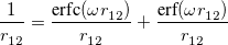
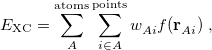
The quadrature approach in Q-Chem is generally similar to that found in many DFT programs. The multi-center XC integrals are first partitioned into “atomic” contributions using a nuclear weight function. Q-Chem uses the nuclear partitioning of Becke [142], though without the “atomic size adjustments” of Ref. Becke:1988a. The atomic integrals are then evaluated through standard one-center numerical techniques. Thus, the exchange-correlation energy is obtained as
 |
(4.52) |
where the function  is the aforementioned XC integrand and the quantities
  are the quadrature weights. The sum over
  runs over grid points belonging to atom
  , which are located at positions
  , so this approach requires only the choice of a suitable one-center integration grid (to define the
  ), which is independent of nuclear configuration. These grids are implemented in Q-Chem in a way that ensures that the
  is rotationally-invariant, i.e., that is does not change when the molecule undergoes rigid rotation in space [143].
Quadrature grids are further separated into radial and angular parts. Within Q-Chem, the radial part is usually treated by the Euler-Maclaurin scheme proposed by Murry et al. [144], which maps the semi-infinite domain  onto
onto  and applies the extended trapezoid rule to the transformed integrand. Alternatively, Gill and Chien [145] proposed a radial scheme based on a Gaussian quadrature on the interval
 ![$[0,1]$](images/img-0182.png) with a different weight function. This “MultiExp" radial quadrature is exact for integrands that are a linear combination of a geometric sequence of exponential functions, and is therefore well suited to evaluating atomic integrals.
with a different weight function. This “MultiExp" radial quadrature is exact for integrands that are a linear combination of a geometric sequence of exponential functions, and is therefore well suited to evaluating atomic integrals.
4.4.5.1 Angular Grids
For a fixed value of the radial spherical-polar coordinate  , a function
  has an exact expansion in spherical harmonic functions,
 |
(4.53) |
Angular quadrature grids are designed to integrate  for fixed , and are often characterized by their degree, meaning the maximum value of
  for which the quadrature is exact, as well as by their efficiency, meaning the number of spherical harmonics exactly integrated per degree of freedom in the formula. Q-Chem supports the following two types of angular grids.
Lebedev grids. These are specially-constructed grids for quadrature on the surface of a sphere [146, 147, 148, 149], based on the octahedral point group. Lebedev grids available in Q-Chem are listed in Table 4.3. These grids typically have near-unit efficiencies, with efficiencies exceeding unity in some cases. A Lebedev grid is selected by specifying the number of grid points (from Table 4.3) using the $rem keyword XC_GRID, as discussed below.
No. Points
Degree
No. Points
Degree
No. Points
Degree
(
 )
) (
) (
) 6
3
230
25
1730
71
14
5
266
27
2030
77
26
7
302
29
2354
83
38
9
350
31
2702
89
50
11
434
35
3074
95
74
13
590
41
3470
101
86
15
770
47
3890
107
110
17
974
53
4334
113
146
19
1202
59
4802
119
170
21
1454
65
5294
125
194
23
Table 4.3: Lebedev angular quadrature grids available in Q-Chem.Gauss-Legendre grids. These are spherical direct-product grids in the two spherical-polar angles,
 and
and  . Integration in over is performed using a Gaussian quadrature derived from the Legendre polynomials, while integration over is performed using equally-spaced points. A Gauss-Legendre grid is selected by specifying the total number of points,
  , to be used for the integration, which specifies a grid consisting of
  points in and
  in , for a degree of
  . Gauss-Legendre grids exhibit efficiencies of only 2/3, and are thus lower in quality than Lebedev grids for the same number of grid points, but have the advantage that they are defined for arbitrary (and arbitrarily-large) numbers of grid points. This offers a mechanism to achieve arbitrary accuracy in the angular integration, if desired.
Combining these radial and angular schemes yields an intimidating selection of quadratures, so it is useful to standardize the grids. This is done for the convenience of the user, to facilitate comparisons in the literature, and also for developers wishing to compared detailed results between different software programs, because the total electronic energy is sensitive to the details of the grid, just as it is sensitive to details of the basis set. Standard quadrature grids are discussed next.
4.4.5.2 Standard Quadrature Grids
The SG-0 [150] and SG-1 [151] standard quadrature grids were designed to match the accuracy of large, dense quadrature grids but with as few points as possible for the sake of computational efficiency. This is accomplished by reducing the number of angular points in regions where sophisticated angular quadrature is not necessary, such as near the nuclei where the charge density is nearly spherically symmetric and at long distance from the nuclei where it varies slowly. A large number of points is retained in the valence region where angular accuracy is critical.
SG-1 dervies from a Euler-Maclaurin-Lebedev-(50,194) grid, meaning one with 50 radial quadrature points and 194 angular points per radial point. This grid has been found to give numerical integration errors of the order of 0.2 kcal/mol for medium-sized molecules, including particularly demanding test cases such as isomerization reactions. This error is deemed acceptable since it is significantly smaller than the accuracy typically achieved by DFT or indeed other quantum-chemical methods. In SG-1, the total number of points is reduced to approximately 1/4 of that of the original EML-(50,194) grid, yet total energies typically change by no more than a few hartree ( kcal/mol) as compared to EML-(50,194). This is the default grid in Q-Chem since v. 3.2.
The SG-0 grid was derived in similar fashion from a MultiExp-Lebedev-(23,170) grid, i.e., using a different radial quadrature as compared to SG-1. SG-0 was pruned while ensuring the error in the computed exchange energies for the atoms and a selection of small molecules was not larger than the corresponding error associated with SG-1. Root-mean-square errors in atomization energies for the molecules in the G1 data set is only 72 hartree with respect to SG-1 [150], while relative energies are also expected to be reproduced well. If absolute energies are being sought, a larger grid is recommended. The SG-0 grid is implemented in Q-Chem for atoms from H to Ar, except for He and Na where SG-1 grid points are used. Please note that SG-0 was re-optimized for Q-Chem v. 3.0, so results may differ slightly as compared to older versions of the program.
Both the SG-0 and SG-1 grids were optimized so that the error in the energy when using the grid did not exceed a target threshold, but derivatives of the energy [including such properties as (hyper)polarizabilities [152]] are often more sensitive to the quality of the integration grid. Special care is required, for example, when imaginary vibrational frequencies are encountered, as low-frequency (but real) vibrational frequencies can manifest as imaginary if the grid is sparse. If imaginary frequencies are found, or if there is some doubt about the frequencies reported by Q-Chem, the recommended procedure is to perform the geometry optimization and vibrational frequency calculations again using a larger grid. (The optimization should converge quite quickly if the previously-optimized geometry is used as an initial guess.)
Finally, it should be noted that both SG-0 and SG-1 were developed at a time when GGAs and hybrid functionals ruled the DFT world. Meta-GGAs, with their dependence on the kinetic energy density [ in Eq. eq:tau] can be much more sensitive to the quality of the integration grid [141]. Specific recommendations for the choice of integration grid when using these functionals can be found in Ref. Mardirossian:2014.
4.4.5.3 Consistency Check and Cutoffs
Whenever Q-Chem calculates numerical density functional integrals, the electron density itself is also integrated numerically as a test of the quality of the numerical quadrature. The extent to which this numerical result differs from the number of electrons is an indication of the accuracy of the other numerical integrals. A warning message is printed whenever the relative error in the numerical electron count reaches 0.01%, indicating that the numerical XC results may not be reliable. If the warning appears on the first SCF cycle it is probably not serious, because the initial-guess density matrix is sometimes not idempotent. This is the case with the SAD guess discussed in Section 4.5, and also with a density matrix that is taken from a previous geometry optimization cycle, and in such cases the problem will likely correct itself in subsequent SCF iterations. If the warning persists, however, then one should consider either using a finer grid or else selecting an alternative initial guess.
By default, Q-Chem will estimate the magnitude of various XC contributions on the grid and eliminate those determined to be numerically insignificant. Q-Chem uses specially-developed cutoff procedures which permits evaluation of the XC energy and potential in only  work for large molecules. This is a significant improvement over the formal
  scaling of the XC cost, and is critical in enabling DFT calculations to be carried out on very large systems. In rare cases, however, the default cutoff scheme can be too aggressive, eliminating contributions that should be retained; this is almost always signaled by an inaccurate numerical density integral. An example of when this could occur is in calculating anions with multiple sets of diffuse functions in the basis. A remedy may be to increase the size of the quadrature grid.
4.4.6 Range-Separated Hybrid Density Functionals
Whereas RSH functionals such as LRC-PBE are attempts to add 100% LR Hartree-Fock exchange with minimal perturbation to the original functional (PBE, in this example), other RSH functionals are of a more empirical nature and their range-separation parameters have been carefully parameterized along with all of the other parameters in the functional. These cases are functionals are discussed first, in Section 4.4.6.1, because their range-separation parameters should be taken as fixed. User-defined values of the range-separation parameter are discussed in Section 4.4.6.2, and Section 4.4.6.3 discusses a procedure for which an optimal, system-specific value of this parameter ( or ) can be chosen for functionals such as LRC-PBE or LRC-PBE.
4.4.6.1 Semi-Empirical RSH Functionals
Semi-empirical RSH functionals for which the range-separation parameter should be considered fixed include the B97, B97X, and B97X-D functionals developed by Chai and Head-Gordon [29, 37]; B97X-V and B97M-V from Mardirossian and Head-Gordon [115, 82]; M11 from Peverati and Truhlar [122]; B97X-D3, M05-D, and M06-D3 from Chai and coworkers [123, 116]; and the screened exchange functionals N12-SX and MN12-SX from Truhlar and co-workers [121]. More recently, Mardirossian and Head-Gordon developed two RSH functionals, B97X-V and B97M-V, via a combinatorial approach by screening over 100,000 possible functionals in the first case and over 10 billion possible functionals in the second case. Both of the latter functionals use the VV10 non-local correlation functional in order to improve the description of non-covalent interactions and isomerization energies. B97M-V is a 12-parameter meta-GGA with 15% short-range exact exchange and 100% long-range exact exchange and is one of the most accurate functionals available through rung 4 of Jacob’s Ladder, across a wide variety of applications. This has been verified by benchmarking the functional on nearly 5000 data points against over 100 alternative functionals available in Q-Chem [82].
4.4.6.2 User-Defined RSH Functionals
As pointed out in Ref. Dreuw:2003 and elsewhere, the description of charge-transfer excited states within density functional theory (or more precisely, time-dependent DFT, which is discussed in Section 6.3) requires full (100%) non-local HF exchange, at least in the limit of large donor–acceptor distance. Hybrid functionals such as B3LYP [154] and PBE0 [155] that are well-established and in widespread use, however, employ only 20% and 25% HF exchange, respectively. While these functionals provide excellent results for many ground-state properties, they cannot correctly describe the distance dependence of charge-transfer excitation energies, which are enormously underestimated by most common density functionals. This is a serious problem in any case, but it is a catastrophic problem in large molecules and in non-covalent clusters, where TDDFT often predicts a near-continuum of spurious, low-lying charge transfer states [156, 157]. The problems with TDDFT’s description of charge transfer are not limited to large donor–acceptor distances, but have been observed at  2 separation, in systems as small as uracil–(HO)
 [156]. Rydberg excitation energies also tend to be substantially underestimated by standard TDDFT.
One possible avenue by which to correct such problems is to parameterize functionals that contain 100% HF exchange, though few such functionals exist to date. An alternative option is to attempt to preserve the form of common GGAs and hybrid functionals at short range (i.e., keep the 25% HF exchange in PBE0) while incorporating 100% HF exchange at long range, which provides a rigorously correct description of the long-range distance dependence of charge-transfer excitation energies, but aims to avoid contaminating short-range exchange-correlation effects with additional HF exchange. The separation is accomplished using the range-separation ansatz that was introduced in Section 4.4.3. In particular, functionals that use 100% HF exchange at long range [ in Eq. eq:RSHGGA] are known as “long-range-corrected” (LRC) functionals. An LRC version of PBE0 would, for example, have
  .
.
To fully specify an LRC functional, one must choose a value for the range separation parameter in Eq. (). In the limit  , the LRC functional in Eq. eq:RSHGGA reduces to a non-RSH functional where there is no “SR” or “LR”, because all exchange and correlation energies are evaluated using the full Coulomb operator, . Meanwhile the
  limit corresponds to a new functional,
  . Full HF exchange is inappropriate for use with most contemporary GGA correlation functionals, so the latter limit is expected to perform quite poorly. Values of
  bohr are likely not worth considering, according to benchmark tests [158, 119].
Evaluation of the short- and long-range HF exchange energies is straightforward [159], so the crux of any RSH functional is the form of the short-range GGA exchange functional, and several such functionals are available in Q-Chem. These include short-range variants of the B88 and PBE exchange described by Hirao and co-workers [47, 118], called B88 and PBE in Q-Chem [160], and an alternative formulation of short-range PBE exchange proposed by Scuseria and co-workers [55], which is known as PBE. These functionals are available in Q-Chem thanks to the efforts of the Herbert group [119, 120]. By way of notation, the terms “PBE”, “PBE”, etc., refer only to the short-range exchange functional,  in Eq. eq:RSHGGA. These functionals could be used in “screened exchange” mode, as described in Section 4.4.3, as for example in the HSE03 functional [161], therefore the designation “LRC-PBE”, for example, should only be used when the short-range exchange functional PBE is combined with 100% Hartree-Fock exchange in the long range.
In general, LRC-DFT functionals have been shown to remove the near-continuum of spurious charge-transfer excited states that appear in large-scale TDDFT calculations [158]. However, certain results depend sensitively upon the value of the range-separation parameter [158, 119, 120, 157, 162], especially in TDDFT calculations (Section 6.3) and therefore the results of LRC-DFT calculations must therefore be interpreted with caution, and probably for a range of values. This can be accomplished by requesting a functional that contains some short-range GGA exchange functional (PBE or PBE, in the examples mentioned above), in combination with setting the $rem variable LRC_DFT = TRUE, which requests the addition of 100% Hartree-Fock exchange in the long-range. Basic job-control variables and an example can be found below. The value of the range-separation parameter is then controlled by the variable OMEGA, as shown in the examples below.
LRC_DFT
Controls the application of long-range-corrected DFT
TYPE:
LOGICAL
DEFAULT:
FALSE
OPTIONS:
FALSE (or 0)
Do not apply long-range correction.
TRUE (or 1)
Add 100% long-range Hartree-Fock exchange to the requested functional.
RECOMMENDATION:
The $rem variable OMEGA must also be specified, in order to set the range-separation parameter.
OMEGA
Sets the range-separation parameter,
TYPE:
INTEGER
DEFAULT:
No default
OPTIONS:
Corresponding to
, in units of bohr
RECOMMENDATION:
None
COMBINE_K
Controls separate or combined builds for short-range and long-range K
TYPE:
LOGICAL
DEFAULT:
FALSE
OPTIONS:
FALSE (or 0)
Build short-range and long-range K separately (twice as expensive as a global hybrid)
TRUE (or 1)
Build short-range and long-range K together (
RECOMMENDATION:
Most pre-defined range-separated hybrid functionals in Q-Chem use this feature by default. However, if a user-specified RSH is desired, it is necessary to manually turn this feature on.
Example 4.25 Application of LRC-BOP to  .
.
$comment
The value of omega is 0.47 by default but can
be overwritten by specifying OMEGA.
$end

$molecule
-1 2
O           1.347338    -0.017773    -0.071860
H           1.824285     0.813088     0.117645
H           1.805176    -0.695567     0.461913
O          -1.523051    -0.002159    -0.090765
H          -0.544777    -0.024370    -0.165445
H          -1.682218     0.174228     0.849364
$end

$rem
   EXCHANGE      LRC-BOP
   BASIS         6-31(1+,3+)G*
   LRC_DFT       TRUE
   OMEGA         300      ! = 0.300 bohr**(-1)
$end
Recently, Rohrdanz et al. [120] have published a thorough benchmark study of both ground- and excited-state properties, using the “LRC-PBEh” functional, in which the “h” indicates a short-range hybrid (i.e., the presence of some short-range HF exchange). Empirically-optimized parameters of  [see Eq. eq:RSHGGA] and
  bohr were obtained [120], and these parameters are taken as the defaults for LRC-PBEh. Caution is warranted, however, especially in TDDFT calculations for large systems, as excitation energies for states that exhibit charge-transfer character can be rather sensitive to the precise value of .Lange:2009,Rohrdanz:2009 In such cases (and maybe in general), the “tuning” procedure described in Section 4.4.6.3 is recommended.
Example 4.26 Application of LRC-PBEh to the  –
– dimer at 5 separation.
$comment
    This example uses the "optimal" parameter set discussed above.
    It can also be run by setting METHOD = LRC-wPBEh.
$end

$molecule
0 1
C           0.670604    0.000000    0.000000
C          -0.670604    0.000000    0.000000
H           1.249222    0.929447    0.000000
H           1.249222   -0.929447    0.000000
H          -1.249222    0.929447    0.000000
H          -1.249222   -0.929447    0.000000
C           0.669726    0.000000    5.000000
C          -0.669726    0.000000    5.000000
F           1.401152    1.122634    5.000000
F           1.401152   -1.122634    5.000000
F          -1.401152   -1.122634    5.000000
F          -1.401152    1.122634    5.000000
$end

$rem
   EXCHANGE      GEN
   BASIS         6-31+G*
   LRC_DFT       TRUE
   OMEGA         200      ! = 0.2 a.u.
   CIS_N_ROOTS   4
   CIS_TRIPLETS  FALSE
$end

$xc_functional
    C PBE    1.00
    X wPBE  0.80
    X HF        0.20
$end
Both LRC functionals and also the asymptotic corrections that will be discussed in Section 4.4.9.1 are thought to reduce self-interaction error in approximate DFT. A convenient way to quantify—or at least depict—this error is by plotting the DFT energy as a function of the (fractional) number of electrons,  , because
  should in principle consist of a sequence of line segments with abrupt changes in slope (the so-called derivative discontinuity [163, 164]) at integer values of , but in practice these plots bow away from straight-line segments [163]. Examination of such plots has been suggested as a means to adjust the fraction of short-range exchange in an LRC functional [165], while the range-separation parameter is tuned as described in Section 4.4.6.3.
Example 4.27 Example of a DFT job with a fractional number of electrons. Here, we make the  anion of fluoride by subracting a fraction of an electron from the HOMO of F
 .
.
$comment
    Subtracting a whole electron recovers the energy of F-.
    Adding electrons to the LUMO is possible as well.
$end

$rem
exchange            b3lyp
basis               6-31+G*
fractional_electron -500  ! /divide by 1000 to get the fraction, -0.5 here.
$end

$molecule
-2 2
F
$end
4.4.6.3 Tuned RSH Functionals
Whereas the range-separation parameters for the functionals described in Section 4.4.6.1 are wholly empirical in nature and should not be adjusted, for the functionals described in Section 4.4.6.2 some adjustment was suggested, especially for TDDFT calculations and for any properties that require interpretation of orbital energies, e.g., HOMO/LUMO gaps. This adjustment can be performed in a non-empirical, albeit system-specific way, by “tuning” the value of in order to satisfy certain criteria that ought rigorously to be satisfied by an exact density functional.
System-specific optimization of is based on the Koopmans condition that would be satisfied for the exact density functional, namely, that for an -electron molecule [166]
 |
(4.54) |
In other words, the HOMO eigenvalue should be equal to minus the ionization energy (IE), where the latter is defined by a  SCF procedure [167, 168]. When an RSH functional is used, all of the quantities in Eq. eq:IP-tuning are -dependent, so this parameter is adjusted until the condition in Eq. eq:IP-tuning is met, which requires a sequence of SCF calculations on both the neutral and ionized species, using different values of . For proper description of charge-transfer states, Baer and co-workers [166] suggest finding the value of that (to the extent possible) satisfies both Eq. eq:IP-tuning for the neutral donor molecule and its analogue for the anion of the acceptor species. Note that for a given approximate density functional, there is no guarantee that the IE condition can actually be satisfied for any value of , but in practice it usually can be, and published benchmarks suggest that this system-specific approach affords the most accurate values of IEs and TDDFT excitation energies [169, 170, 166]. It should be noted, however, that the optimal value of can very dramatically with system size, e.g., it is very different for the cluster anion (HO)
 than it is for cluster (HO)
 [162].
A script that optimizes , called OptOmegaIPEA.pl, is located in the $QC/bin directory. The script scans over the range 0.1–0.8 bohr, corresponding to values of the $rem variable OMEGA in the range 100–800. See the script for the instructions how to modify the script to scan over a wider range. To execute the script, you need to create three inputs for a BNL job using the same geometry and basis set, for a neutral molecule (N.in), its anion (M.in), and its cation (P.in), and then run the command
OptOmegaIPEA.pl >& optomega
which both generates the input files (N_*, P_*, M_*) and runs Q-Chem on them, writing the optimization output into optomega. This script applies the IE condition to both the neutral molecule and its anion, minimizing the sum of  for these two species. A similar script, OptOmegaIP.pl, uses Eq. eq:IP-tuning for the neutral molecule only.
Note: (i) If the system does not have positive EA, then the tuning should be done according to the IP condition only. The IP/EA script will yield an incorrect value of in such cases.
(ii) In order for the scripts to work, one must specify SCF_FINAL_PRINT = 1 in the inputs. The scripts look for specific regular expressions and will not work correctly without this keyword.
(iii) When tuning we recommend taking the amount of BNL exchange to be 1.0 and not 0.9
Although the tuning procedure was originally developed by Baer and co-workers using the BNL functional [169, 170, 166], it has more recently been applied using functionals such as LRC-PBE (see, e.g., Ref. Uhlig:2014), and the scripts will work with functionals other than BNL. The $xc_functional keyword for a BNL calculation reads:
$xc_functional
  X HF 1.0
  X BNL 0.9
  C LYP 1.0
$end
and the $rem keyword reads
$rem
  EXCHANGE      GENERAL
  SEPARATE_JK   TRUE
  OMEGA         500     != 0.5 Bohr$^{-1}$
  DERSCREEN     FALSE   ! if performing unrestricted calculation
  IDERIV        0       ! if performing unrestricted Hessian evaluation
$end
4.4.7 DFT Methods for van der Waals Interactions
This section describes three different procedures for obtaining a better description of dispersion (i.e., van der Waals) interactions DFT calculations: non-local correlation functionals (Section 4.4.7.1), empirical atom–atom dispersion potentials (“DFT-D”, Section 4.4.7.2), and finally the Becke-Johnson exchange-dipole model (XDM, Section 4.4.7.3).
4.4.7.1 Non-Local Correlation (NLC) Functionals
Q-Chem includes four non-local correlation functionals that describe long-range dispersion:
vdW-DF-04, developed by Langreth, Lundqvist, and coworkers [35, 36], implemented as described in Ref. Vydrov:2008.
vdW-DF-10 (also known as vdW-DF2), which is a re-parameterization [172] of vdW-DF-04, implemented in the same way as its precursor.
VV09, developed [33] and implemented [173] by Vydrov and Van Voorhis.
VV10 by Vydrov and Van Voorhis [34].
All of these functionals are implemented self-consistently and analytic gradients with respect to nuclear displacements are available [171, 173, 34]. The non-local correlation is governed by the $rem variable NL_CORRELATION, which can be set to one of the four values: vdW-DF-04, vdW-DF-10, VV09, or VV10. Note that the vdW-DF-04, vdW-DF-10, and VV09 functionals are used in combination with LSDA correlation, which must be specified explicitly. For instance, vdW-DF-10 is invoked by the following keyword combination:
CORRELATION        PW92
NL_CORRELATION     vdW-DF-10
VV10 is used in combination with PBE correlation, which must be added explicitly. In addition, the values of two parameters,  and
and  must be specified for VV10. These parameters are controlled by the $rem variables NL_VV_C and NL_VV_B, respectively. For instance, to invoke VV10 with
  and
and  , the following input is used:
CORRELATION        PBE
NL_CORRELATION     VV10
NL_VV_C            93
NL_VV_B            590
The variable NL_VV_C may also be specified for VV09, where it has the same meaning. By default,  is used in VV09 (i.e. NL_VV_C is set to 89). However, in VV10 neither nor are assigned a default value and must always be provided in the input.
Unlike local (LSDA) and semilocal (GGA and meta-GGA) functionals, for non-local functionals evaluation of the correlation energy requires a double integral over the spatial variables [cf. Eq. ()]:
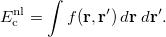 |
(4.55) |
In practice, this double integration is performed numerically on a quadrature grid [171, 173, 34]. By default, the SG-1 quadrature (described in Section 4.4.5.2 below) is used to evaluate  , but a different grid can be requested via the $rem variable NL_GRID. The non-local energy is rather insensitive to the fineness of the grid, so that SG-1 or even SG-0 grids can be used in most cases. However, a finer grid may be required for the (semi)local parts of the functional, as controlled by the XC_GRID variable and discussed in Section 4.4.5.2.
Several exchange-correlation functionals in Q-Chem are pre-defined to use the VV10 non-local correlation functional. The two functionals from the original paper[34] can be used by specifying METHOD = VV10 or METHOD LC-VV10. In addition, the combinatorially-optimized functionals of Mardirossian and Head-Gordon (B97X-V, B97M-V, and B97M-V) use non-local correlation and can be invoked by setting METHOD to wB97X-V, B97M-V, or wB97M-V.
Example 4.28 Geometry optimization of the methane dimer using VV10 with rPW86 exchange.
$molecule
0 1
C   0.000000  -0.000140   1.859161
H  -0.888551   0.513060   1.494685
H   0.888551   0.513060   1.494685
H   0.000000  -1.026339   1.494868
H   0.000000   0.000089   2.948284
C   0.000000   0.000140  -1.859161
H   0.000000  -0.000089  -2.948284
H  -0.888551  -0.513060  -1.494685
H   0.888551  -0.513060  -1.494685
H   0.000000   1.026339  -1.494868
$end

$rem
JobType            Opt
BASIS              aug-cc-pVTZ
EXCHANGE           rPW86
CORRELATION        PBE
XC_GRID            75000302
NL_CORRELATION     VV10
NL_GRID            1
NL_VV_C            93
NL_VV_B            590
$end
In the above example, an EML-(75,302) grid is used to evaluate the rPW86 exchange and PBE correlation, but a coarser SG-1 grid is used for the non-local part of VV10. Furthermore, the above example is identical to specifying METHOD = VV10.
NL_CORRELATION
Specifies a non-local correlation functional that includes non-empirical dispersion.
TYPE:
STRING
DEFAULT:
None
No non-local correlation.
OPTIONS:
None
No non-local correlation
vdW-DF-04
the non-local part of vdW-DF-04
vdW-DF-10
the non-local part of vdW-DF-10 (also known as vdW-DF2)
VV09
the non-local part of VV09
VV10
the non-local part of VV10
RECOMMENDATION:
Do not forget to add the LSDA correlation (PW92 is recommended) when using vdW-DF-04, vdW-DF-10, or VV09. VV10 should be used with PBE correlation. Choose exchange functionals carefully: HF, rPW86, revPBE, and some of the LRC exchange functionals are among the recommended choices.
NL_VV_C
Sets the parameter
coefficients.
TYPE:
INTEGER
DEFAULT:
89
for VV09
No default
for VV10
OPTIONS:
Corresponding to

RECOMMENDATION:
NL_VV_B
Sets the parameter
TYPE:
INTEGER
DEFAULT:
No default
OPTIONS:
Corresponding to

RECOMMENDATION:
The optimal value depends strongly on the exchange functional used.
4.4.7.2 Empirical Dispersion Corrections: DFT-D
There are currently three unique DFT-D methods in Q-Chem, which are requested via the $rem variable DFT_D, and which are discussed below.
DFT_D
Controls the empirical dispersion correction to be added to a DFT calculation.
TYPE:
LOGICAL
DEFAULT:
None
OPTIONS:
FALSE
(or 0) Do not apply the DFT-D2, DFT-CHG, or DFT-D3(0) scheme
EMPIRICAL_GRIMME
DFT-D2 dispersion correction from Grimme
EMPIRICAL_CHG
DFT-CHG dispersion correction from Chai and Head-Gordon
EMPIRICAL_GRIMME3
DFT-D3(0) dispersion correction from Grimme
RECOMMENDATION:
NONE
Thanks to the efforts of the Sherrill group, Grimm’s popular DFT-D2 empirical dispersion correction [28] is available in Q-Chem, along with analytic gradients and frequencies. This correction can be added to any density functional that is available in Q-Chem, although its use with the non-local correlation functionals discussed in Section 4.4.7.1 is obviously not recommended.
DFT-D2 adds an extra term,
 |
 |
(4.56) | ||
 |
 |
(4.57) | ||
 |
![$\displaystyle = \left[1+e^{-d(R_{AB}/R_{AB}^0 - 1)}\right]^{-1} $](images/img-0235.png) |
(4.58) |
where  is a global scaling parameter (near unity) and
  is a damping function meant to help avoid double-counting correlation effects at short range (and to prevent the divergence of
  ), which depends on another parameter,
  . The quantity
  is the sum of the van der Waals radii of atoms A and B. Grimme has suggested using
  for PBE,
  for BLYP,
  for BP86, and
  for B3LYP, and these are the default values when those functionals are used. Otherwise, the default value is
  .
.
DFT-D2 parameters, including the atomic van der Waals radii, can be altered using a $empirical_dispersion input section. For example:
$empirical_dispersion
S6 1.1
D 10.0
C6 Ar 4.60 Ne 0.60
VDW_RADII Ar 1.60 Ne 1.20
$end
Any values not specified explicitly will default to the values optimized by Grimme.
Note: (i) DFT-D2 is only defined for elements up to Xe.
(ii) B97-D is an exchange-correlation functional that automatically employs the DFT-D2 dispersion correction when used via METHOD B97-D.
An alternative to Grimme’s DFT-D2 is the empirical dispersion correction of Chai and Head-Gordon [37], which employs a slightly different damping function
![$\displaystyle \label{eqn:CHG} f_{\rm damp}(R_{AB}) = \left[1+a(R_{AB}/R_{AB}^0)^{-12}\right]^{-1} $](images/img-0246.png) |
(4.59) |
The Chai–Head-Gordon dispersion correction is activated by setting DFT_D = EMPIRICAL_CHG, and the damping parameter  is controlled by the keyword DFT_D_A.
DFT_D_A
Controls the strength of dispersion corrections in the Chai–Head-Gordon DFT-D scheme, Eq. eqn:CHG.
TYPE:
INTEGER
DEFAULT:
600
OPTIONS:
Corresponding to
.
RECOMMENDATION:
Use the default.
Note: (i) DFT-CHG is only defined for elements up to Xe.
(ii) The B97X-D and M05-D functionals automatically employ the DFT-CHG dispersion correction when used via METHOD = wB97X-D or wM05-D.
Finally, Grimme’s more recent DFT-D3 method [38], and improvement on his DFT-D2 approach, [28] is available along with analytic first and second derivatives, and can be combined with any of the density functionals available in Q-Chem. The total DFT-D3 energy is given by  , where
  is the total energy from KS-DFT and the dispersion correction
  is a sum of two- and three-body energies. Currently, only the original “zero-damping” version of DFT-D3, DFT-D3(0), is available in Q-Chem.
DFT-D3 is requested by setting DFT_D = EMPIRICAL_GRIMME3. The model depends on four scaling factors [,  ,
,  and
and  , as defined in Eq. (4) of Ref. Grimme:2010], which can be adjusted using the $rem variables described below. By fixing
  , the other three factors were optimized for several functionals (see Table IV in Ref. Grimme:2010). For example,
  and
and  were optimized for PBE, versus
  and
and  for B3LYP. For most functionals, is set to 1. By default, Q-Chem loads the parameters found here:
for the following functionals: B1B95, B3LYP, BLYP, BP86, PBE, PBE0, PW6B95, PWB6K, revPBE, TPSS, TPSSh, MPW1B95, MPWB1K, B3PW91, BMK, CAM-B3LYP, and revPBE0. Otherwise, the default values of , , and are 1.0.
Note: (i) DFT-D3(0) is defined for elements up to Pu ( ).
).
(ii) The B97-D3(0), B97X-D3, M06-D3 functionals automatically employ the DFT-D3(0) dispersion correction when invoked by setting METHOD equal to B97-D3, wB97X-D3, or wM06-D3.
DFT_D3_S6
Controls the strength of dispersion corrections,
TYPE:
INTEGER
DEFAULT:
1000
OPTIONS:
Corresponding to
.
RECOMMENDATION:
NONE
DFT_D3_RS6
Controls the strength of dispersion corrections, s
, in the Grimme’s DFT-D3(0) method (see Table IV in Ref. Grimme:2010).
TYPE:
INTEGER
DEFAULT:
1000
OPTIONS:
Corresponding to
.
RECOMMENDATION:
NONE
DFT_D3_S8
Controls the strength of dispersion corrections,
TYPE:
INTEGER
DEFAULT:
1000
OPTIONS:
Corresponding to
.
RECOMMENDATION:
NONE
DFT_D3_RS8
Controls the strength of dispersion corrections,
TYPE:
INTEGER
DEFAULT:
1000
OPTIONS:
Corresponding to
.
RECOMMENDATION:
NONE
The three-body interaction term [38],  , must be explicitly turned on, if desired.
DFT_D3_3BODY
Controls whether the three-body interaction in Grimme’s DFT-D3 method should be applied (see Eq. (14) in Ref. Grimme:2010).
TYPE:
LOGICAL
DEFAULT:
FALSE
OPTIONS:
FALSE (or 0)
Do not apply the three-body interaction term
TRUE
Apply the three-body interaction term
RECOMMENDATION:
NONE
Example 4.29 Applications of B3LYP-D3 to a methane dimer.
$comment
Geometry optimization, followed by single-point calculations
using a larger basis set.
$end

$molecule
0 1
C       0.000000    -0.000323     1.755803
H      -0.887097     0.510784     1.390695
H       0.887097     0.510784     1.390695
H       0.000000    -1.024959     1.393014
H       0.000000     0.001084     2.842908
C       0.000000     0.000323    -1.755803
H       0.000000    -0.001084    -2.842908
H      -0.887097    -0.510784    -1.390695
H       0.887097    -0.510784    -1.390695
H       0.000000     1.024959    -1.393014
$end

$rem
jobtype         opt
exchange        B3LYP
basis           6-31G*
DFT_D           EMPIRICAL_GRIMME3
DFT_D3_S6       1000
DFT_D3_RS6      1261
DFT_D3_S8       1703
DFT_D3_3BODY    FALSE
$end

@@@

$molecule
READ
$end

$rem
jobtype         sp
exchange        B3LYP
basis           6-311++G**
DFT_D           EMPIRICAL_GRIMME3
DFT_D3_S6       1000
DFT_D3_RS6      1261
DFT_D3_S8       1703
DFT_D3_3BODY    FALSE
$end
4.4.7.3 Exchange-Dipole Model (XDM)
Becke and Johnson have proposed a conceptually simple yet accurate dispersion model called the exchange-dipole model (XDM) [133, 174]. In this model the dispersion attraction emerges from the interaction between the instantaneous dipole moment of the exchange hole in one molecule and the induced dipole moment in another. It is a conceptually simple but powerful approach that has been shown to yield very accurate dispersion coefficients without fitting parameters. This allows the calculation of both intermolecular and intramolecular dispersion interactions within a single DFT framework. The implementation and validation of this method in the Q-Chem code is described in Ref. Kong:2009.
Fundamental to the XDM model is the calculation of the norm of the dipole moment of the exchange hole at a given point:
 |
(4.60) |
where  labels the spin and
  is the exchange-hole function. The XDM version that is implemented in Q-Chem employs the Becke-Roussel (BR) model exchange-hole function. In previous work on the BR model,
  was not available in analytical form and one had to determine its value numerically at each grid point. Q-Chem has developed for the first time an analytical expression for this function based on non-linear interpolation and spline techniques, which greatly improves efficiency as well as the numerical stability [175].
There are two different damping functions used in the XDM model of Becke and Johnson. One of them uses only the intermolecular dispersion coefficient, and its implementation in Q-Chem is denoted as "XDM6". In this version the dispersion energy is computed as
 |
(4.61) |
where  is a universal parameter,
  is the distance between atoms and
  , and
, and  is the sum of the absolute values of the correlation energies of the free atoms and . The dispersion coefficients
  is computed as
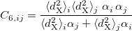 |
(4.62) |
where  is the exchange-hole dipole moment of the atom, and
  is the effective polarizability of the atom in the molecule.
The XDM6 scheme can be further generalized to include higher-order dispersion coefficients, which leads to the “XDM10” model in Q-Chem, whose dispersion energy is
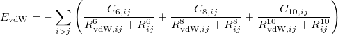 |
(4.63) |
where ,  and
and  are dispersion coefficients computed using higher-order multipole moments of the exchange hole, including dipole, quadrupole and octupole) [176]. The quantity
  is the sum of the effective vdW radii of atoms and , which is a linear function
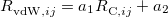 |
(4.64) |
of the so called critical distance  between atoms and , computed according to
![\begin{equation} R_{{\rm C},ij}^{{}} = \frac{1}{3}\left[ \left(\frac{C_{8,ij}}{C_{6,ij}}\right)^{1/2} +\left(\frac{C_{10,ij}}{C_{6,ij}}\right)^{1/4} +\left(\frac{C_{10,ij}}{C_{8,ij}}\right)^{1/2} \right] \; . \end{equation}](images/img-0285.png) |
(4.65) |
In the XDM10 scheme there are two universal parameters,  and
and  . Their default values of 0.83 and 1.35, respectively, are due to Johnson and Becke [174], determined by least-squares fitting to the binding energies of a set of intermolecular complexes. These values are not the only possible optimal set to use with XDM. Becke’s group later suggested several other XC functional combinations with XDM that employ different values of and . The user is advised to consult the recent literature for details [177, 178].
The computed vdW energy  is added as a post-SCF correction. Analytic gradients and Hessians are available for both XDM6 and XDM10. Additional job control and customization options are listed below.
DFTVDW_JOBNUMBER
Basic vdW job control
TYPE:
INTEGER
DEFAULT:
0
OPTIONS:
0
Do not apply the XDM scheme.
1
add vdW as energy/gradient correction to SCF.
2
add vDW as a DFT functional and do full SCF (this option only works with XDM6).
RECOMMENDATION:
none
DFTVDW_METHOD
Choose the damping function used in XDM
TYPE:
INTEGER
DEFAULT:
1
OPTIONS:
1
use Becke’s damping function including
2
use Becke’s damping function with higher-order (
and
) terms.
RECOMMENDATION:
none
DFTVDW_MOL1NATOMS
The number of atoms in the first monomer in dimer calculation
TYPE:
INTEGER
DEFAULT:
0
OPTIONS:
0–

RECOMMENDATION:
none
DFTVDW_KAI
Damping factor
TYPE:
INTEGER
DEFAULT:
800
OPTIONS:
10–1000
RECOMMENDATION:
none
DFTVDW_ALPHA1
Parameter in XDM calculation with higher-order terms
TYPE:
INTEGER
DEFAULT:
83
OPTIONS:
10-1000
RECOMMENDATION:
none
DFTVDW_ALPHA2
Parameter in XDM calculation with higher-order terms.
TYPE:
INTEGER
DEFAULT:
155
OPTIONS:
10-1000
RECOMMENDATION:
none
DFTVDW_USE_ELE_DRV
Specify whether to add the gradient correction to the XDM energy. only valid with Becke’s
TYPE:
LOGICAL
DEFAULT:
1
OPTIONS:
1
use density correction when applicable.
0
do not use this correction (for debugging purposes).
RECOMMENDATION:
none
DFTVDW_PRINT
Printing control for VDW code
TYPE:
INTEGER
DEFAULT:
1
OPTIONS:
0
no printing.
1
minimum printing (default)
2
debug printing
RECOMMENDATION:
none
Example 4.30 Sample input illustrating a frequency calculation of a vdW complex consisted of He atom and N molecule.
$molecule

0 1
He .0 .0 3.8
N .000000 .000000 0.546986
N .000000 .000000 -0.546986
$end

$rem
JOBTYPE		FREQ
IDERIV			2
EXCHANGE		B3LYP
INCDFT			0
SCF_CONVERGENCE	8
BASIS				6-31G*
!vdw parameters settings
DFTVDW_JOBNUMBER		1
DFTVDW_METHOD			1
DFTVDW_PRINT			0
DFTVDW_KAI				800
DFTVDW_USE_ELE_DRV	0
$end
XDM can be used in conjunction with different GGA, meta-GGA pure or hybrid functionals, even though the original implementation of Becke and Johnson was in combination with HF exchange, or with a specific meta-GGA exchange and correlation (the BR89 exchange and BR94 correlation functionals). For example, encouraging results have been obtained using XDM with B3LYP [175]. Becke has found more recently that this model can be efficiently combined with the P86 exchange functional, with the hyper-GGA functional B05. Using XDM together with PBE exchange plus LYP correlation, or PBE exchange plus BR94 correlation, has been also found fruitful.
4.4.8 Double-Hybrid Density Functional Theory
The recent advance in double-hybrid density functional theory (DH-DFT) [126, 179, 180, 181, 124], has demonstrated its great potential for approaching the chemical accuracy with a computational cost comparable to the second-order Møller-Plesset perturbation theory (MP2). In a DH-DFT, a Kohn-Sham (KS) DFT calculation is performed first, followed by a treatment of non-local orbital correlation energy at the level of second-order Møller-Plesset perturbation theory (MP2) [182]. This MP2 correlation correction includes a a same-spin (ss) component,  , as well as an opposite-spin (os) component,
  , which are added to the total energy obtained from the KS-DFT calculation. Two scaling parameters,
  and
and  , are introduced in order to avoid double-counting correlation:
 |
(4.66) |
A starting point for understanding where a functional form like Eq. eq:dft2a might come from is the adiabatic connection formula that provides a rigorous way to define double-hybrid functionals. One considers an adiabatic path between the fictitious noninteracting Kohn-Sham reference system ( ) and the real physical system (
 ), while holding the electron density fixed at its value for the real system, for all
  . Then
![\begin{equation} \label{sung1} E_{\rm XC} \left[\rho \right]=\int _{0}^{1}U_{{\rm XC},\lambda }[\rho ] \; d\lambda \, , \end{equation}](images/img-0300.png) |
(4.67) |
where  is the exchange-correlation energy at a coupling strength , meaning that the exchange-correlation energy if the electron–electron terms in the Hamiltonian had the form
  rather than
  . Using a linear model of this quantity,
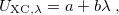 |
(4.68) |
one obtains the popular hybrid functional that includes the HF exchange (or occupied orbitals) such as B3LYP [31]. If one further uses the Gorling-Levy’s perturbation theory (GL2) to define the initial slope at = 0, one obtains the doubly hybrid functional form in Eq. eq:dft2a that includes MP2 type perturbative terms (PT2) involving virtual Kohn-Sham orbitals [183]:
 |
(4.69) |
The adiabatic connection formula has been used to develop double hybrid functionals such as XYG3 [124]. Note that XYG3, as implemented in Q-Chem, uses B3LYP orbitals to generate the density and evaluate the PT2 terms. This is different from B2PLYP, an earlier doubly hybrid functional from Grimme [126]. The latter uses truncated Kohn-Sham orbitals while XYG3 uses converged KS orbitals to evaluate the PT2 terms. The performance of XYG3 is not only comparable to that of the G2 or G3 theory for thermochemistry, but barrier heights and non-covalent interactions, including stacking interactions, are also very well described by XYG3 [124]. The recommended basis set for XYG3 is 6-311+G(3df,2p).
Due to the inclusion of PT2 terms, the cost of double-hybrid calculations is formally  , as in conventional MP2, thereby not applicable to large systems and partly losing DFT’s cost advantages. However, the highly successful SOS-MP2 and local SOS-MP2 algorithms in Q-Chem can be leveraged to develop double-hybrid functionals based on these
  methods. A version of XYG3 that uses SOS-MP2 is the XYGJ-OS functional [125]. This functional has 4 parameters that are optimized using thermochemical data. It is not only faster than XYG3, but comparable to XYG3 (or perhaps slightly better) in accuracy. If the local SOS-MP2 algorithm is applied, the scaling of XYGJ-OS is further reduced to . Recently, XYGJ-OS became the first double-hybrid functional whose analytic energy gradient has been derived and implemented [184].
Other more empirical double-hybrid functionals have been implemented in Q-Chem. Among the B97 series of functionals, B97X-2 [129] is a long-range corrected double hybrid that can greatly reduce the self-interaction errors (due to its high fraction of HF exchange), and has been shown significantly superior to other functionals for systems with both bonded and non-bonded interactions. Due to the sensitivity of PT2 correlation energy with respect to the choices of basis sets, B97X-2 was parameterized with two different basis sets: the B97X-2(LP) was parameterized for use with 6-311++G(3df,3pd), while B97X-2(TQZ) was parameterized with the T/Q (triple- /quadruple-) extrapolation to the basis set limit. A careful reading of Ref. Chai:2009 is highly advised before using either of these two functionals.
Job control variables for double-hybrid DFT are described below. Note that the PT2 correlation energy can also be computed with the efficient resolution-of-identity (RI) methods; see Section 5.5.
DH
Controls the application of DH-DFT scheme.
TYPE:
LOGICAL
DEFAULT:
FALSE
OPTIONS:
FALSE (or 0)
Do not apply the DH-DFT scheme
TRUE (or 1)
Apply DH-DFT scheme
RECOMMENDATION:
NONE
The following to $rem variables pertain to the B97X-2(LP) and B97X-2(TQZ) functionals.
SSS_FACTOR
Controls the strength of the same-spin component of PT2 correlation energy.
TYPE:
INTEGER
DEFAULT:
0
OPTIONS:
Corresponding to
in Eq. (4.66).
RECOMMENDATION:
NONE
SOS_FACTOR
Controls the strength of the opposite-spin component of PT2 correlation energy.
TYPE:
INTEGER
DEFAULT:
0
OPTIONS:
Corresponding to
in Eq. (4.66).
RECOMMENDATION:
NONE
Example 4.31 Applications of B2PLYP functional to LiH.
$comment
Single-point calculation on LiH without RI, followed by a
single-point calculation with RI.
$end

$molecule
0 1
H
Li H 1.6
$end

$rem
jobtype         sp
exchange        B2PLYP
basis           cc-pvtz
$end

@@@

$molecule
READ
$end

$rem
jobtype         sp
exchange        B2PLYP
basis           cc-pvtz
aux_basis       rimp2-cc-pvtz
$end
Example 4.32 Application of B97X-2(TQZ) functional (with and without RI) to LiH molecules.
$comment
Single-point calculation on LiH (with RI).
$end

$molecule
0 1
H
Li H 1.6
$end

$rem
jobtype         sp
exchange        omegaB97X-2(TQZ)
basis           cc-pvqz
aux_basis       rimp2-cc-pvqz
$end

@@@

$comment
Single-point calculation on LiH (without RI).
$end

$molecule
READ
$end

$rem
jobtype		sp
exchange		omegaB97X-2(TQZ)
basis		cc-pvqz
$end
In the following example of XYG3, Q-Chem automatically performs a the B3LYP calculation first, then uses the resulting orbitals to evaluate the PT2 correlation terms. Once can also use XYG3 combined with the RI approximation; use EXCHANGE = XYG3RI to do so, along with an appropriate choice of auxiliary basis set.
Example 4.33 XYG3 calculation of N
$molecule
0 1
 N     0.00000000    0.00000000    0.54777500
 N     0.00000000    0.00000000   -0.54777500
$end

$rem
 exchange	xyg3
 basis	6-311+G(3df,2p)
$end
The next example illustrates XYGJ-OS. This functional uses the RI approximation by default, so it is necessary to specify an auxiliary basis set.
Example 4.34 XYGJ-OS calculation of N
$molecule
0 1
 N      0.00000000    0.00000000    0.54777500
 N      0.00000000    0.00000000   -0.54777500
$end

$rem
 exchange	xygjos
 basis	6-311+G(3df,2p)
 aux_basis	rimp2-cc-pVtZ
 purecart	1111
 time_mp2	true
$end
The final example uses the local version of XYGJ-OS, which is the same as the original XYGJ-OS but with the use of the attenuated Coulomb metric to solve the RI coefficients. Here, the keyword omega determines the locality of the metric.
Example 4.35 Local XYGJ-OS calculation of N
$molecule
0 1
 N    0.000    0.000   0.54777500
 N    0.000    0.000  -0.54777500
$end

$rem
 exchange   lxygjos
 omega   200
 basis   6-311+G(3df,2p)
 aux_basis   rimp2-cc-pVtZ
 purecart   1111
$end
4.4.9 Asymptotically Corrected Exchange-Correlation Potentials
No GGA exchange functional can simultaneously produce the correct contribution to the exchange energy density and exchange potential in the asymptotic region of molecular systems [185], and existing GGA exchange-correlation (xc) potentials decay much faster than the correct  xc potential in the asymptotic region [186]. High-lying occupied orbitals and low-lying virtual orbitals are therefore too loosely bound, and
  becomes far smaller than the ionization energy, despite the exact condition that these should be the same for the exact functional [167, 168]. Moreover, response properties may be poorly predicted from TDDFT calculations with GGA functionals [167]. Long-range corrected hybrid DFT (LRC-DFT), described in Section 4.4.6, has greatly remedied this situation, but is more expensive that KS-DFT with GGA functionals due to the use of Hatree-Fock exchange. The asymptotic corrections described in this section are designed to remedy the same problems but within the GGA framework.
4.4.9.1 LB94 Scheme
An asymptotically corrected (AC) exchange potential proposed by van Leeuwen and Baerends is [185]
 |
(4.70) |
where  is the reduced density gradient. For an exponentially-decaying density, this potential reduces to in the asymptotic region of molecular systems. The LB94 xc potential is formed by a linear combination of LDA xc potential and the LB exchange potential [185]:
 |
(4.71) |
The parameter in Eq. eq:vx_LB was determined by fitting to the exact xc potential for Be atom. As mentioned in Refs. Casida:1998 and Hirata:1999b, for TDDFT calculations, it is sufficient to include the AC xc potential for ground-state calculations followed by TDDFT calculations with an adiabatic LDA xc kernel. The implementation of the LB94 xc potential in Q-Chem takes this approach, using the LB94 xc potential for the ground state calculations, followed by a TDDFT calculation with an adiabatic LDA xc kernel. This TDLDA/LB94 approach has been widely applied to study excited-state properties of large molecules.
Since the LB exchange potential in Eq. eq:vx_LB does not come from the functional derivative of an exchange energy functional, the Levy-Perdew virial relation [189] is used instead to obtain the exchange energy:
![\begin{equation} E_ x^{\text {LB}} = -\int v_ x^{\text {LB}}([\rho ],\textbf{r})[3\rho (\textbf{r})+\textbf{r}\hat\nabla \rho (\textbf{r})]d\textbf{r} \end{equation}](images/img-0313.png) |
(4.72) |
An LB94 calculation is requested by setting EXCHANGE = LB94 in the $rem section. Additional job control and examples appear below.
LB94_BETA
Sets the
TYPE:
INTEGER
DEFAULT:
500
OPTIONS:
Corresponding to
.
RECOMMENDATION:
Use the default.
Example 4.36 Applications of LB94 xc potential to N molecule.
$comment
TDLDA/LB94 calculation is performed for excitation energies.
$end

$molecule
0 1
N	0.0000	0.0000	0.0000
N	1.0977	0.0000	0.0000
$end

$rem
jobtype = sp
exchange = lb94
basis = 6-311(2+,2+)G**
cis_n_roots = 30
rpa = true
$end
4.4.9.2 Localized Fermi-Amaldi (LFA) Schemes
Another alternative, proposed by Pan, Fang and Chai [190], is to use a localized version of Fermi-Amaldi exchange-correlation functional. The resulting exchange density functional, whose functional derivative has the correct asymptotic behavior, can be directly added to any semilocal density functional. Three variants of this method were proposed in Ref. Chai:2013b. The simplest of these, the strictly-localized Fermi-Amaldi (LFAs) scheme, is implemented in Q-Chem, for molecules consisting of atoms with  .
.
Example 4.37 LFAs-PBE single-point TD-DFT calculation with water molecule
$comment
Use LFAs-PBE potential for ground-state calculations, followed by
TDDFT calculations with an adiabatic PBE xc kernel.
$end

$molecule
   0  1
   O
   H1  O  oh
   H2  O  oh  H1  hoh

   oh  =   1.0
   hoh = 110.0
$end.

$rem
jobtype     sp
exchange    gen
basis       6-311(2+,2+)G**
cis_n_roots 30
rpa         true
$end

$xc_functional
X PBE   1.0
C PBE   1.0
X LFAs  1.0
$end
4.4.10 Derivative Discontinuity Restoration
From the perspective of perturbation theory, Chai and Chen [191] proposed a systematic procedure for the evaluation of the derivative discontinuity of the exchange-correlation energy functional in KS-DFT, wherein the exact derivative discontinuity can in principle be obtained by summing up all the perturbation corrections to infinite order. Truncation of the perturbation series at low order yields an efficient scheme for obtaining the approximate derivative discontinuity. In particular, the first-order correction term is equivalent to the frozen-orbital approximation method. Its implementation in Q-Chem supports only local and GGA functionals at present, not meta-GGA, hybrid, or non-local functionals. Job control variables and examples appear below.
FOA_FUNDGAP
Compute the frozen-orbital approximation of the fundamental gap.
TYPE:
Boolean
DEFAULT:
FALSE
OPTIONS:
FALSE
Do not compute FOA derivative discontinuity and fundamental gap.
TRUE
Compute and print FOA fundamental gap information. Implies KS_GAP_PRINT.
RECOMMENDATION:
Use in conjuction with KS_GAP_UNIT if true.
Example 4.38 frozen-orbital approximation of derivative discontinuity with PBE and LFAs-PBE functionals on carbon atom
$comment
Frozen-orbital derivative discontinuity, C atom, PBE
$end

$molecule
0 3
C
$end

$rem
jobtype           sp
basis             6-31G*
method            PBE
foa_fundgap       true
ks_gap_unit       1 ! print gap info in eV
$end

@@@

$comment
with LFAs-PBE functional instead
$end

$molecule
READ
$end

$rem
jobtype           sp
basis             6-31G*
scf_guess         READ
exchange          gen
foa_fundgap       true
ks_gap_unit       1
$end

$xc_functional
X PBE  1.0
X LFAs 1.0
C PBE  1.0
$end
4.4.11 Thermally-Assisted-Occupation Density Functional Theory (TAO-DFT)
Aiming to study the ground-state properties of large, strongly correlated systems with minimum computational complexity, Prof. Jeng-Da Chai recently developed thermally-assisted-occupation density functional theory (TAO-DFT) [192]. Unlike conventional multireference methods, the computational complexity of TAO-DFT increases very insignificantly with the size of the active space (i.e., an active space restriction is not needed for TAO-DFT calculations), and TAO-DFT appears to be very promising for the study of large poly-radical systems. TAO-DFT is a DFT scheme with fractional orbital occupations produced by the Fermi-Dirac distribution, controlled by a fictitious temperature , and existing XC functionals (e.g., LDA or GGAs) can be used in TAO-DFT [193]. The computational cost of the method is similar to that of KS-DFT for single-point energy calculations and analytical nuclear gradients, and reduces to the cost of KS-DFT in the absence of strong static correlation effects.
There are several $rem variables that are used for TAO-DFT.
TAO_DFT
Controls whether to use TAO-DFT.
TYPE:
Boolean
DEFAULT:
false
OPTIONS:
false
Do not use TAO-DFT
true
Use TAO-DFT
RECOMMENDATION:
NONE
TAO_DFT_THETA
Controls the value of the fictitious temperature
TYPE:
INTEGER
DEFAULT:
7
OPTIONS:
(hartrees), where
RECOMMENDATION:
NONE
TAO_DFT_THETA_NDP
Controls the value of the fictitious temperature
TYPE:
INTEGER
DEFAULT:
3
OPTIONS:
RECOMMENDATION:
NONE
Note that setting TAO_DFT_THETA = 0 recovers ordinary KS-DFT [192]. In addition to the xc functional, a functional ![$E_{\theta }[\rho ]$](images/img-0317.png) is needed in TAO-DFT. Currently available in Q-Chem are an LDA version [192] (the ETheta_LDA functional) as well as a version based on the gradient expansion approximation (GEA) [193] (ETheta_GEA functional), and the latter may be substituted for the former in the sample jobs below.
is needed in TAO-DFT. Currently available in Q-Chem are an LDA version [192] (the ETheta_LDA functional) as well as a version based on the gradient expansion approximation (GEA) [193] (ETheta_GEA functional), and the latter may be substituted for the former in the sample jobs below.
Example 4.39 TAO-LDA calcuation on Be atom
$molecule
0 1
Be
$end

$rem
jobtype           sp
basis             6-31G*
exchange          gen
tao_dft           true
tao_dft_theta     7  ! default, theta=7 mhartree
tao_dft_theta_ndp 3  ! default
$end

$xc_functional
X   S             1.0
C   PW92          1.0
X   ETheta_LDA    1.0
$end
Example 4.40 TAO-PBE, spin-restricted calculation on stretched N
$comment
Spin-restricted calculation on stretched N2
$end

$molecule
0 1
N1
N2 N1 5
$end

$rem
jobtype           sp
basis             6-31G*
exchange          gen
tao_dft           true
tao_dft_theta     40  ! theta = 40 mhartree
tao_dft_theta_ndp 3
$end

$xc_functional
X PBE         1.0
C PBE         1.0
X ETheta_LDA  1.0
$end
Example 4.41 TAO-PBE, spin-unrestricted calculation on stretched N
$comment
Spin-unrestricted optimization calculation on stretched N2
$end
$molecule
0 1
N1
N2 N1 5
$end
$rem
jobtype           opt
unrestricted      true
basis             6-31G*
exchange          gen
tao_dft           true
tao_dft_theta     40  ! theta = 40 mhartrees
tao_dft_theta_ndp 3   ! can omit this line
scf_guess         gwh
SCF_GUESS_MIX     3   ! mix in 30% LUMO in alpha to break symmetry
$end
$xc_functional
X PBE         1.0
C PBE         1.0
X ETheta_LDA  1.0
$end