10.11 Intracules
The many dimensions of electronic wavefunctions makes them difficult to analyze and interpret. It is often convenient to reduce this large number of dimensions, yielding simpler functions that can more readily provide chemical insight. The most familiar of these is the one-electron density  , which gives the probability of an electron being found at the point
  . Analogously, the one-electron momentum density
  gives the probability that an electron will have a momentum of
  . However, the wavefunction is reduced to the one-electron density much information is lost. In particular, it is often desirable to retain explicit two-electron information. Intracules are two-electron distribution functions and provide information about the relative position and momentum of electrons. A detailed account of the different type of intracules can be found in Ref. Gill:2003. Q-Chem’s intracule package was developed by Aaron Lee and Nick Besley, and can compute the following intracules for or HF wavefunctions:
Position intracules,
 : describes the probability of finding two electrons separated by a distance
  .
. Momentum intracules,
 : describes the probability of finding two electrons with relative momentum
  .
. Wigner intracule,
 : describes the combined probability of finding two electrons separated by and with relative momentum .
10.11.1 Position Intracules
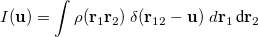
The intracule density,  , represents the probability for the inter-electronic vector
  :
:
 |
(10.13) |
where  is the two-electron density. A simpler quantity is the spherically averaged intracule density,
 |
(10.14) |
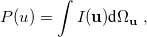
where  is the angular part of
  , measures the probability that two electrons are separated by a scalar distance
  . This intracule is called a position intracule [501]. If the molecular orbitals are expanded within a basis set
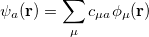 |
(10.15) |
The quantity can be expressed as
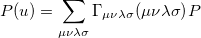 |
(10.16) |
where  is the two-particle density matrix and
  is the position integral
 |
(10.17) |
and  ,
,  ,
,  and
and  are basis functions. For HF wavefunctions, the position intracule can be decomposed into a Coulomb component,
 |
(10.18) |
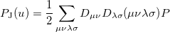
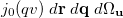
and an exchange component,
![\begin{equation} P_\ensuremath{\mathrm{}}{K}(u) = -\frac{1}{2} \sum _{\mu \nu \lambda \sigma } \left[ D_{\mu \lambda }^\alpha D_{\nu \sigma }^\alpha + D_{\mu \lambda }^\beta D_{\nu \sigma }^\beta \right] ({\mu \nu \lambda \sigma })_\ensuremath{\mathrm{}}{P} \end{equation}](images/img-1229.png) |
(10.19) |
where  etc. are density matrix elements. The evaluation of ,
  and
and  within Q-Chem has been described in detail in Ref. Lee:1999.
Some of the moments of are physically significant [503], for example
 |
 |
 |
(10.20) | ||
 |
|
 |
(10.21) | ||
 |
|
 |
(10.22) | ||
 |
|
 |
(10.23) |
where  is the number of electrons and,
  is the electronic dipole moment and
  is the trace of the electronic quadrupole moment tensor. Q-Chem can compute both moments and derivatives of position intracules.
10.11.2 Momentum Intracules
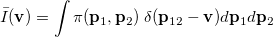
Analogous quantities can be defined in momentum space;  , for example, represents the probability density for the relative momentum
  :
:
 |
(10.24) |
where  momentum two-electron density. Similarly, the spherically averaged intracule
 |
(10.25) |
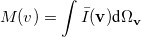
where  is the angular part of , is a measure of relative momentum
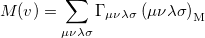
  and is called the momentum intracule. The quantity can be written as
 |
(10.26) |
where  is the two-particle density matrix and
  is the momentum integral [504]
 |
(10.27) |
The momentum integrals only possess four-fold permutational symmetry, i.e.,
 |
(10.28) | ||
 |
(10.29) |
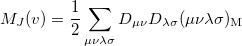
and therefore generation of is roughly twice as expensive as . Momentum intracules can also be decomposed into Coulomb  and exchange
  components:
 |
(10.30) |
![\begin{equation} M_{\ensuremath{\mathrm{K}}}(v) = -\frac{1}{2} \sum \limits _{\mu \nu \lambda \sigma } \left[ D_{\mu \lambda }^\alpha D_{\nu \sigma }^\alpha + D_{\mu \lambda }^\beta D_{\nu \sigma }^\beta \right] (\mu \nu \lambda \sigma )_{\ensuremath{\mathrm{M}}} \end{equation}](images/img-1258.png) |
(10.31) |
Again, the even-order moments are physically significant [504]:
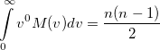 |
(10.32) |
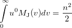 |
(10.33) |
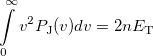 |
(10.34) |
 |
(10.35) |
where is the number of electrons and  is the total electronic kinetic energy. Currently, Q-Chem can compute , and using
  and
and  basis functions only. Moments are generated using quadrature and consequently for accurate results must be computed over a large and closely spaced range.
10.11.3 Wigner Intracules
The intracules and provide a representation of an electron distribution in either position or momentum space but neither alone can provide a complete description. For a combined position and momentum description an intracule in phase space is required. Defining such an intracule is more difficult since there is no phase space second-order reduced density. However, the second-order Wigner distribution [505],
 |
(10.36) |
can be interpreted as the probability of finding an electron at  with momentum
  and another electron at
  with momentum
  . [The quantity
  is often referred to as “quasi-probability distribution” since it is not positive everywhere.]
The Wigner distribution can be used in an analogous way to the second order reduced densities to define a combined position and momentum intracule. This intracule is called a Wigner intracule, and is formally defined as
 |
(10.37) |
If the orbitals are expanded in a basis set, then can be written as
 |
(10.38) |
where ( is the Wigner integral
 |
(10.39) |
Wigner integrals are similar to momentum integrals and only have four-fold permutational symmetry. Evaluating Wigner integrals is considerably more difficult that their position or momentum counterparts. The fundamental ![$\left[ssss\right]_{\ensuremath{\mathrm{w}}}$](images/img-1274.png) integral,
integral,
![$\displaystyle \left[ssss\right]_{\ensuremath{\mathrm{W}}} $](images/img-1275.png) |
|
![$\displaystyle \frac{u^2v^2}{2\pi ^2}\; \int \int \exp \left[-\alpha |\ensuremath{\mathbf{r}}\! -\! \ensuremath{\mathbf{A}}|^2 -\! \beta |\ensuremath{\mathbf{r}}\! +\! \ensuremath{\mathbf{q}}\! -\! \ensuremath{\mathbf{B}}|^2 -\! \gamma |\ensuremath{\mathbf{r}}\! +\! \ensuremath{\mathbf{q}}\! +\! \ensuremath{\mathbf{u}}\! -\! \ensuremath{\mathbf{C}}|^2 -\! \delta |\ensuremath{\mathbf{r}}\! +\! \ensuremath{\mathbf{u}}\! -\! \ensuremath{\mathbf{D}}|^2 \right] \times \nonumber $](images/img-1276.png) |
|||
 |
|
 |
(10.40) |
can be expressed as
![\begin{equation} \left[ssss\right]_{\ensuremath{\mathrm{W}}} = \frac{\pi u^2 v^2\; e^{-(R+\lambda ^2 u^2 +\mu ^2 v^2)}}{ 2(\alpha +\delta )^{3/2}(\beta +\gamma )^{3/2}}\int {e^{-\ensuremath{\mathbf{P}}\cdot \ensuremath{\mathbf{u}}}} j_0 \left(|\ensuremath{\mathbf{Q}}+\eta \ensuremath{\mathbf{u}}|v \right)\; d\Omega _ u \end{equation}](images/img-1278.png) |
(10.41) |
or alternatively
![\begin{equation} \left[ssss\right]_{\ensuremath{\mathrm{W}}} = \frac{2\pi ^2 u^2 v^2 e^{-(R+\lambda ^2 u^2+\mu ^2 v^2)}}{(\alpha +\delta )^{3/2}(\beta +\gamma )^{3/2}} \sum \limits _{n=0}^\infty (2n+1) i_ n(P\, u) j_ n(\eta u v) j_ n(Q v) P_ n \left( {\frac{\ensuremath{\mathbf{P}}\cdot \ensuremath{\mathbf{Q}}}{P\; Q}} \right) \end{equation}](images/img-1279.png) |
(10.42) |
Two approaches for evaluating  have been implemented in Q-Chem, full details can be found in Ref. Wigner:1932. The first approach uses the first form of
 ![$\left[ssss\right]_{\ensuremath{\mathrm{W}}}$](images/img-1281.png) and used Lebedev quadrature to perform the remaining integrations over . For high accuracy large Lebedev grids [157, 155, 507] should be used, grids of up to 5294 points are available in Q-Chem. Alternatively, the second form can be adopted and the integrals evaluated by summation of a series. Currently, both methods have been implemented within Q-Chem for and basis functions only.
and used Lebedev quadrature to perform the remaining integrations over . For high accuracy large Lebedev grids [157, 155, 507] should be used, grids of up to 5294 points are available in Q-Chem. Alternatively, the second form can be adopted and the integrals evaluated by summation of a series. Currently, both methods have been implemented within Q-Chem for and basis functions only.
When computing intracules it is most efficient to locate the loop over and/or points within the loop over shell-quartets [508]. However, for this requires a large amount of memory to store all the integrals arising from each  point. Consequently, an additional scheme, in which the and points loop is outside the shell-quartet loop, is available. This scheme is less efficient, but substantially reduces the memory requirements.
10.11.4 Intracule Job Control
The following $rem variables can be used to control the calculation of intracules.
INTRACULE
Controls whether intracule properties are calculated (see also the $intracule section).
TYPE:
LOGICAL
DEFAULT:
FALSE
OPTIONS:
FALSE
No intracule properties.
TRUE
Evaluate intracule properties.
RECOMMENDATION:
None
WIG_MEM
Reduce memory required in the evaluation of
TYPE:
LOGICAL
DEFAULT:
FALSE
OPTIONS:
FALSE
Do not use low memory option.
TRUE
Use low memory option.
RECOMMENDATION:
The low memory option is slower, use default unless memory is limited.
WIG_LEB
Use Lebedev quadrature to evaluate Wigner integrals.
TYPE:
LOGICAL
DEFAULT:
FALSE
OPTIONS:
FALSE
Evaluate Wigner integrals through series summation.
TRUE
Use quadrature for Wigner integrals.
RECOMMENDATION:
None
WIG_GRID
Specify angular Lebedev grid for Wigner intracule calculations.
TYPE:
INTEGER
DEFAULT:
194
OPTIONS:
Lebedev grids up to 5810 points.
RECOMMENDATION:
Larger grids if high accuracy required.
N_WIG_SERIES
Sets summation limit for Wigner integrals.
TYPE:
INTEGER
DEFAULT:
10
OPTIONS:

RECOMMENDATION:
Increase
N_I_SERIES
Sets summation limit for series expansion evaluation of
.
TYPE:
INTEGER
DEFAULT:
40
OPTIONS:

RECOMMENDATION:
Lower values speed up the calculation, but may affect accuracy.
N_J_SERIES
Sets summation limit for series expansion evaluation of
.
TYPE:
INTEGER
DEFAULT:
40
OPTIONS:
RECOMMENDATION:
Lower values speed up the calculation, but may affect accuracy.
10.11.5 Format for the $intracule Section
int_type |
0 |
Compute |
1 |
Compute |
|
2 |
Compute |
|
3 |
Compute |
|
4 |
Compute |
|
5 |
Compute |
|
6 |
Compute |
|
u_points |
Number of points, start, end. |
|
v_points |
Number of points, start, end. |
|
moments |
0–4 |
Order of moments to be computed ( |
derivs |
0–4 |
order of derivatives to be computed ( |
accuracy |
|
( |
 specify accuracy of intracule interpolation table (
 Example 10.220 Compute HF/STO-3G , and for Ne, using Lebedev quadrature with 974 point grid.
$molecule
   0  1
   Ne
$end

$rem
   METHOD      hf
   BASIS       sto-3g
   INTRACULE   true
   WIG_LEB     true
   WIG_GRID    974
$end

$intracule
   int_type   3
   u_points  10   0.0  10.0
   v_points   8   0.0   8.0
   moments    4
   derivs     4
   accuracy   8
$end
Example 10.221 Compute HF/6-31G intracules for H O using series summation up to =25 and 30 terms in the series evaluations of and .
$molecule
   0  1
   H1
   O   H1  r
   H2  O   r  H1  theta

   r = 1.1
   theta = 106
$end

$rem
   METHOD         hf
   BASIS          6-31G
   INTRACULE      true
   WIG_MEM        true
   N_WIG_SERIES   25
   N_I_SERIES     40
   N_J_SERIES     50
$end

$intracule
   int_type    2
   u_points   30   0.0   15.0
   v_points   20   0.0   10.0
$end