10.17 Calculating the Population of Effectively Unpaired Electrons with DFT
In a stretched hydrogen molecule the two electrons that are paired at equilibrium forming a bond become un-paired and localized on the individual H atoms. In singlet diradicals or doublet triradicals such a weak paring exists even at equilibrium. At a single-determinant SCF level of the theory the valence electrons of a singlet system like H remain perfectly paired, and one needs to include non-dynamical correlation to decouple the bond electron pair, giving rise to a population of effectively-unpaired (“odd”, radicalized) electrons [633, 634, 635]. When the static correlation is strong, these electrons remain mostly unpaired and can be described as being localized on individual atoms.
These phenomena can be properly described within wave-function formalism. Within DFT, these effects can be described by broken-symmetry approach or by using SF-TDDFT (see Section 6.3.1). Below we describe how to derive this sort of information from pure DFT description of such low-spin open-shell systems without relying on spin-contaminated solutions.
The first-order reduced density matrix (1-RDM) corresponding to a single-determinant wave function (e.g., SCF or Kohn-Sham DFT) is idempotent:
 |
(10.113) |
where  is the electron density of spin
  at position
  , and
, and  is the spin-resolved 1-RDM of a single Slater determinant. The cross product
 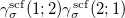 reflects the Hartree-Fock exchange (or Kohn-Sham exact-exchange) governed by the HF exchange hole:
 |
(10.114) |
When 1-RDM includes electron correlation, it becomes nonidempotent:
 |
(10.115) |
The function  measures the deviation from idempotency of the correlated 1-RDM and yields the density of effectively-unpaired (odd) electrons of spin at point
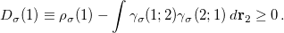
  [633, 636]. The formation of effectively-unpaired electrons in singlet systems is therefore exclusively a correlation based phenomenon. Summing over the spin components gives the total density of odd electrons, and integrating the latter over space gives the mean total number of odd electrons
  :
:
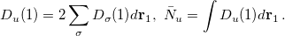 |
(10.116) |
The appearance of a factor of 2 in Eq. (10.116) above is required for reasons discussed in reference [636]. In Kohn-Sham DFT, the SCF 1-RDM is always idempotent which impedes the analysis of odd electron formation at that level of the theory. Ref. [637] has proposed a remedy to this situation. It was noted that the correlated 1-RDM cross product entering Eq. (10.115) reflects an effective exchange (also known as cumulant exchange [634]). The KS exact-exchange hole is itself artificially too delocalized. However, the total exchange-correlation interaction in a finite system with strong left-right (i.e., static) correlation is normally fairly localized, largely confined within a region of roughly atomic size [638]. The effective exchange described with the correlated 1-RDM cross product should be fairly localized as well. With this in mind, the following form of the correlated 1-RDM cross product was proposed [637]:
 |
(10.117) |
where the function  is a model DFT exchange hole of Becke-Roussel (BR) form used in Becke’s B05 method [133]. The latter describes left-right static correlation effects in terms of certain effective exchange-correlation hole [133]. The extra delocalization of the HF exchange hole alone is compensated by certain physically motivated real-space corrections to it [133]:
 |
(10.118) |
where the BR exchange hole  is used in B05 as an auxiliary function, such that the potential from the relaxed BR hole equals that of the exact-exchange hole. This results in relaxed normalization of the auxiliary BR hole less than or equal to 1:
 |
(10.119) |
The expression of the relaxed normalization  is quite complicated, but it is possible to represent it in closed analytic form [135, 136]. The smaller the relaxed normalization
  , the more delocalized the corresponding exact-exchange hole [133]. The
  exchange hole is further deepened by a fraction of the
  exchange hole,
 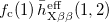 , which gives rise to left-right static correlation. The local correlation factor
  in Eq.(10.118) governs this deepening and hence the strength of the static correlation at each point [133]:
 |
(10.120) |
Using Eqs. (10.120), (10.116), and (10.117), the density of odd electrons becomes:
 |
(10.121) |
The final formulas for the spin-summed odd electron density and the total mean number of odd electrons read:
![\begin{equation} \label{eq:b05-9} D_{u}(1)=4\, a_{\mathrm{nd}}^{\mathrm{op}}\; f_{\mathrm{c}}(1)\left[{\rho }_{\alpha }(1)\, N_{X\beta }^{\mathrm{eff}}(1)+{\rho }_{\beta }(1)\, N_{X\alpha }^{\mathrm{eff}}(1)\right]\; , \; \; {\bar{N}}_{u}=\int \, D_{u}(\mathbf{r_{1}})\; d\mathbf{r_{1}}\, . \end{equation}](images/img-1622.png) |
(10.122) |
Here 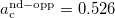 is the SCF-optimized linear coefficient of the opposite-spin static correlation energy term of the B05 functional [133, 136] .
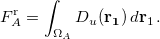
It is informative to decompose the total mean number of odd electrons into atomic contributions. Partitioning in real space the mean total number of odd electrons  as a sum of atomic contributions, we obtain the atomic population of odd electrons (
 ) as:
) as:
 |
(10.123) |
Here  is a subregion assigned to atom
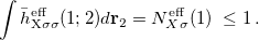
  in the system. To define these atomic regions in a simple way, we use the partitioning of the grid space into atomic subgroups within Becke’s grid-integration scheme [142]. Since the present method does not require symmetry breaking, singlet states are calculated in restricted Kohn-Sham (RKS) manner even at strongly stretched bonds. This way one avoids the destructive effects that the spin contamination has on and on the Kohn-Sham orbitals. The calculation of can be done fully self-consistently only with the RI-B05 and RI-mB05 functionals. In these cases no special keywords are needed, just the corresponding EXCHANGE rem line for these functionals. Atomic population of odd electron can be estimated also with any other functional in two steps: first obtaining a converged SCF calculation with the chosen functional, then performing one single post-SCF iteration with RI-B05 or RI-mB05 functionals reading the guess from a preceding calculation, as shown on the input example below:
Example 10.243 To calculate the odd-electron atomic population and the correlated bond order in stretched H, with B3LYP/RI-mB05, and with fully SCF RI-mB05
$comment
Stretched H2: example of B3LYP calculation of
the atomic population of odd electrons
with post-SCF RI-BM05 extra iteration.
$end

$molecule
0 1
H   0.  0.   0.0
H   0.  0.   1.5000
$end

$rem
JOBTYPE     SP
SCF_GUESS   CORE
METHOD B3LYP
BASIS    G3LARGE
purcar 222
THRESH    14
MAX_SCF_CYCLES   80
PRINT_INPUT     TRUE
SCF_FINAL_PRINT  1
INCDFT    FALSE
XC_GRID 000128000302
SYM_IGNORE    TRUE
SYMMETRY      FALSE
SCF_CONVERGENCE   9
$end

@@@

$comment
Now one RI-B05 extra-iteration after B3LYP
to generate the odd-electron atomic population and the
correlated bond order.
$end

$molecule
READ
$end

$rem
JOBTYPE    SP
SCF_GUESS  READ
EXCHANGE BM05
purcar 22222
BASIS G3LARGE
AUX_BASIS riB05-cc-pvtz
THRESH    14
PRINT_INPUT     TRUE
INCDFT    FALSE
XC_GRID 000128000302
SYM_IGNORE    TRUE
SYMMETRY      FALSE
MAX_SCF_CYCLES   0
SCF_CONVERGENCE   9
dft_cutoffs 0
1415 1
$end

@@@

$comment
Finally, a fully SCF run RI-B05 using the previous output as a guess.
The following input lines are obligatory here:
purcar 22222
AUX_BASIS riB05-cc-pvtz
dft_cutoffs 0
1415 1
$end

$molecule
READ
$end

$rem
JOBTYPE    SP
SCF_GUESS  READ
EXCHANGE BM05
purcar 22222
BASIS G3LARGE
AUX_BASIS riB05-cc-pvtz
THRESH    14
PRINT_INPUT     TRUE
INCDFT    FALSE
IPRINT   3
XC_GRID 000128000302
SYM_IGNORE    TRUE
SCF_FINAL_PRINT  1
SYMMETRY      FALSE
MAX_SCF_CYCLES   80
SCF_CONVERGENCE   8
dft_cutoffs 0
1415 1
$end
Once the atomic population of odd electrons is obtained, a calculation of the corresponding correlated bond order of Mayer’s type follows in the code, using certain exact relationships between ,  , and the correlated bond order of Mayer type
  . Both new properties are printed at the end of the output, right after the multipoles section. It is useful to compare the correlated bond order with Mayer’s SCF bond order. To print the latter, use SCF_FINAL_PRINT = 1.