9.6 Nonadiabatic Couplings and Optimization of Minimum-Energy Crossing Points
9.6.1 Nonadiabatic Couplings
Conical intersections are degeneracies between Born-Oppenheimer potential energy surfaces that facilitate nonadiabatic transitions between excited states, i.e., internal conversion and intersystem crossing processes, both of which represent a breakdown of the Born-Oppenheimer approximation [359, 360]. Although simultaneous intersections between more than two electronic states are possible [359], consider for convenience the two-state case, and let
 |
(9.1) |
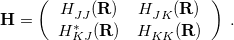
denote the matrix representation of the vibronic (vibrational + electronic) Hamiltonian [Eq. eq:Hamiltonian] in a basis of two electronic states,  and
and  . (Electronic degrees of freedom have been integrated out of this expression, and
  represents the remaining, nuclear coordinates.) By definition, the Born-Oppenheimer states are the ones that diagonalize
  at a particular molecular geometry , and thus two conditions must be satisfied in order to obtain degeneracy in the Born-Oppenheimer representation:
  and
and  . As such, degeneracies between two Born-Oppenheimer potential energy surfaces exist in subspaces of dimension
  , where
  is the number of internal (vibrational) degrees of freedom (assuming the molecule is non-linear). This ()-dimensional subspace is known as the seam space because the two states are degenerate everywhere within this space. In the remaining two degrees of freedom, known as the branching space, the degeneracy between Born-Oppenheimer surfaces is lifted by an infinitesimal displacement, which in a three-dimensional plot resembles a double cone about the point of intersection, hence the name conical intersection.
The branching space is defined by the span of a pair of vectors  and
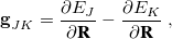
and  . The former is simply the difference in the gradient vectors of the two states in question,
 |
(9.2) |
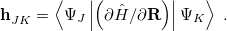
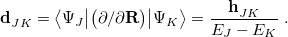
and is readily evaluated at any level of theory for which analytic energy gradients are available (or less-readily, via finite difference, if they are not!). The definition of the nonadiabatic coupling vector , on the other hand, is more involved and not directly amenable to finite-difference calculations:
 |
(9.3) |
This is closely related to the derivative coupling vector
 |
(9.4) |
The latter expression for  demonstrates that the coupling between states becomes large in regions of the potential surface where the two states are nearly degenerate. The relative orientation and magnitudes of the vectors
  and determined the topography around the intersection, i.e., whether the intersection is “peaked” or “sloped”; see Ref. Herbert:2016b for a pedagogical overview.
Algorithms to compute the nonadiabatic couplings are not widely available in quantum chemistry codes, but thanks to the efforts of the Herbert and Subotnik groups, they are available in Q-Chem when the wave functions  and
and  , and corresponding electronic energies
  and
and  , are computed at the CIS or TDDFT level [361, 362, 363, 364], or at the corresponding spin-flip (SF) levels of theory (SF-CIS or SF-TDDFT). The spin-flip implementation [362] is particularly significant, because only that approach—and not traditional spin-conserving CIS or TDDFT—affords correct topology around conical intersections that involve the ground state. To understand why, suppose that in Eq. eq:H_2x2 represents the ground state; call it
  for definiteness. In linear response theory (TDDFT) or in CIS (by virtue of Brillouin’s theorem), the coupling matrix elements between the reference (ground) state and all of the excited states vanish identically, hence
  . This means that there is only one condition to satisfy in order to obtain degeneracy, hence the branching space is one- rather than two-dimensional, for any conical intersection that involves the ground state [486]. (For intersections between two excited states, the topology should be correct.) In the spin-flip approach, however, the reference state has a different spin multiplicity than the target states; if the latter have spin quantum number
  , then the reference state has spin
  . This has the effect that the ground state of interest (spin ) is treated as an excitation, and thus on a more equal footing with excited states of the same spin, and it rigorously fixes the topology problem around conical intersections [362].
Nonadiabatic (derivative) couplings are available for both CIS and TDDFT. The CIS nonadiabatic couplings can be obtained from direct differentiations of the wave functions with respect to nuclear positions [361, 362]. For TDDFT, the same procedure can be carried out to calculate the approximate nonadiabatic couplings, in what has been termed the “pseudo-wave function” approach [487, 362]. Formally more rigorous TDDFT nonadiabatic couplings derived from quadratic response theory are also available, although they are subject to certain undesirable, accidental singularities if for the two states and in Eq. eq:hJK, the energy difference  is quasi-degenerate with the excitation energy
  for some third state,
  [363, 364]. As such, the pseudo-wave function method is the recommended approach for computing nonadiabatic couplings with TDDFT, although in the spin flip case the pseudo-wave function approach is rigorously equivalent to the pseudo-wave function approach, and is free of singularities [363].
Finally, we note that there is some evidence that SF-TDDFT calculations are most accurate when used with functionals containing  50% Hartree-Fock exchange [94, 488], and many studies with this method (see Ref. Herbert:2016b for a survey) have used the BH&HLYP functional, in which LYP correlation is combined with Becke’s “half and half” (BH&H) exchange functional, consisting of 50% Hartree-Fock exchange and 50% Becke88 exchange (EXCHANGE = BHHLYP in Q-Chem.)
9.6.2 Job Control and Examples
In order to perform nonadiabatic coupling calculations, the $derivative_coupling section must be given:
$derivative_couplingNonadiabatic couplings will then be computed between all pairs of the states
one line comment
$end
 ; use “0” to request the HF or DFT reference state, “1” for the first excited state, etc.
CIS_DER_COUPLE
Determines whether we are calculating nonadiabatic couplings.
TYPE:
LOGICAL
DEFAULT:
FALSE
OPTIONS:
TRUE
Calculate nonadiabatic couplings.
FALSE
Do not calculate nonadiabatic couplings.
RECOMMENDATION:
None.
CIS_DER_NUMSTATE
Determines among how many states we calculate nonadiabatic couplings. These states must be specified in the $derivative_coupling section.
TYPE:
INTEGER
DEFAULT:
0
OPTIONS:
0
Do not calculate nonadiabatic couplings.

Calculate
pairs of nonadiabatic couplings.
RECOMMENDATION:
None.
SET_QUADRATIC
Determines whether to include full quadratic response contributions for TDDFT.
TYPE:
LOGICAL
DEFAULT:
FALSE
OPTIONS:
TRUE
Include full quadratic response contributions for TDDFT.
FALSE
Use pseudo-wave function approach.
RECOMMENDATION:
The pseudo-wave function approach is usually accurate enough and is free of accidental singularities. Consult Refs. Zhang:2015a and Ou:2015 for additional guidance.
Example 9.199 Nonadiabatic couplings among the lowest five singlet states of ethylene, computed at the TD-B3LYP level using the pseudo-wave function approach.
$molecule
0 1
 C                  1.85082356   -1.78953123    0.00000000
 H                  2.38603593   -2.71605577    0.00000000
 H                  0.78082359   -1.78977646    0.00000000
 C                  2.52815456   -0.61573833    0.00000000
 H                  1.99294220    0.31078621    0.00000000
 H                  3.59815453   -0.61549310    0.00000000
$end

$rem
jobtype sp
cis_n_roots 4
cis_triplets false
set_iter 50
cis_der_numstate 5
cis_der_couple true
exchange b3lyp
basis 6-31G*
$end

$derivative_coupling
0 is the reference state
0 1 2 3 4
$end
Example 9.200 Nonadiabatic couplings between  and
and  states of ethylene using BH&HLYP and spin-flip TDDFT.
$molecule
0 3
 C                  1.85082356   -1.78953123    0.00000000
 H                  2.38603593   -2.71605577    0.00000000
 H                  0.78082359   -1.78977646    0.00000000
 C                  2.52815456   -0.61573833    0.00000000
 H                  1.99294220    0.31078621    0.00000000
 H                  3.59815453   -0.61549310    0.00000000
$end

$rem
jobtype sp
spin_flip true
unrestricted true
cis_n_roots 4
cis_triplets false
set_iter 50
cis_der_numstate 2
cis_der_couple true
exchange bhhlyp
basis 6-31G*
$end

$derivative_coupling
comment
1 3
$end
Example 9.201 Nonadiabatic couplings between and  states of ethylene computed via quadratic response theory at the TD-B3LYP level.
$molecule
0 1
 C                  1.85082356   -1.78953123    0.00000000
 H                  2.38603593   -2.71605577    0.00000000
 H                  0.78082359   -1.78977646    0.00000000
 C                  2.52815456   -0.61573833    0.00000000
 H                  1.99294220    0.31078621    0.00000000
 H                  3.59815453   -0.61549310    0.00000000
$end

$rem
jobtype sp
cis_n_roots 4
cis_triplets false
rpa true
set_iter 50
cis_der_numstate 2
cis_der_couple true
exchange b3lyp
basis 6-31G*
set_quadratic true #include full quadratic response
$end

$derivative_coupling
comment
1 2
$end
9.6.3 Minimum-Energy Crossing Points
The seam space of a conical intersection is really a (hyper)surface of dimension , and while the two electronic states in question are degenerate at every point within this space, the electronic energy varies from one point to the next. To provide a simple picture of photochemical reaction pathways, it is often convenient to locate the minimum-energy crossing point (MECP) within this  -dimensional seam. Two separate minimum-energy pathway searches, one on the excited state starting from the ground-state geometry and terminating at the MECP, and the other on the ground state starting from the MECP and terminating at the ground-state geometry, then affords a photochemical mechanism. (See Ref. Zhang:2014a for a simple example.) In some sense, then, the MECP is to photochemistry what the transition state is to reactions that occur on a single Born-Oppenheimer potential energy surface. One should be wary of pushing this analogy too far, because whereas a transition state reasonably be considered to be a bottleneck point on the reaction pathway, the path through a conical intersection may be downhill and perhaps therefore more likely to proceed from one surface to the other at a point “near" the intersection, and in addition there can be multiple conical intersections between the same pair of states so more than one photochemical mechanism may be at play. Such complexity could be explored, albeit at significantly increased cost, using nonadiabatic “surface hopping" ab initio molecular dynamics, as described in Section 9.7.6. Here we describe the computationally-simpler procedure of locating an MECP along a conical seam.
Recall that the branching space around a conical intersection between electronic states and is spanned by two vectors, [Eq. eq:gJK] and [Eq. eq:hJK]. While the former is readily available in analytic form for any electronic structure method that has analytic excited-state gradients, the nonadiabatic coupling vector is not available for most methods. For this reason, several algorithms have been developed to optimize MECPs without the need to evaluate , and three such algorithms are available in Q-Chem.
Mart nez and co-workers [490] developed a penalty-constrained MECP optimization algorithm that consists of minimizing the objective function
![\begin{equation} F_\sigma (\mathbf{R}) = \tfrac {1}{2}\bigl [E_ I(\mathbf{R}) + E_ J(\mathbf{R})\bigr ] + \sigma \left(\frac{\bigl [E_ I(\mathbf{R}) - E_ J(\mathbf{R})\bigr ]^2}{E_ I(\mathbf{R}) - E_ J(\mathbf{R}) + \alpha }\right) \; , \end{equation}](images/img-1104.png) |
(9.5) |
where  is a fixed parameter to avoid singularities and
  is a Lagrange multiplier for a penalty function meant to drive the energy gap to zero. Minimization of
  is performed iteratively for increasingly large values .
A second MECP optimization algorithm is a simplification of the penalty-constrained approach that we call the “direct” method. Here, the gradient of the objective function is
 |
(9.6) |
where
 |
(9.7) |
is the mean energy gradient, with  being the nuclear gradient for state
  , and
, and
 |
(9.8) |
is the normalized difference gradient. Finally,
 |
(9.9) |
projects the gradient difference direction out of the mean energy gradient in Eq. eq:direct_MECP. The algorithm then consists in minimizing along the gradient  , with for the iterative cycle over a Lagrange multiplier, which can sometimes be slow to converge.
The third and final MECP optimization algorithm that is available in Q-Chem is the branching-plane updating method developed by Morokuma and co-workers [491] and implemented in Q-Chem by Zhang and Herbert [489]. This algorithm uses a gradient that is similar to that in Eq. eq:direct_MECP but projects out not just  in Eq. eq:MECP_projector1 but also a second vector that is orthogonal to it, representing an iteratively-updated approximation to the branching space.
None of these three methods requires evaluation of nonadiabatic couplings, and all three can be used to optimize MECPs at the CIS, SF-CIS, TDDFT, SF-TDDFT, and SOS-CIS(D0) levels. The direct algorithm can also be used for EOM-XX-CCSD methods (XX = EE, IP, or EA). It should be noted that since EOM-XX-CCSD is a linear response method, it suffers from the same topology problem around conical intersections involving the ground state that was described in regards to TDDFT in Section 9.6.1. With spin-flip approaches, correct topology is obtained [362].
Analytic derivative couplings are available for (SF-)CIS and (SF-)TDDFT, so for these methods one can alternatively employ an optimization algorithm that makes use of both and . Such an algorithm, due to Schlegel and co-workers [492], is available in Q-Chem and consists of optimization along the gradient in Eq. eq:direct_MECP but with a projector
 |
(9.10) |
where
 |
(9.11) |
in place of the projector in Eq. eq:MECP_projector1. Equation eq:MECP_projector2 has the effect of projecting the span of and (i.e., the branching space) out of state-averaged gradient in Eq. eq:direct_MECP. The tends to reduce the number of iterations necessary to converge the MECP, and since calculation of the (optional) vector represents only a slight amount of overhead on top of the (required) vector, this last algorithm tends to yield significant speed-ups relative to the other three [362]. As such, it is the recommended choice for (SF-)CIS and (SF-)TDDFT.
It should be noted that while the spin-flip methods cure the topology problem around conical intersections that involve the ground state, this method tends to exacerbate spin contamination relative to the corresponding spin-conserving approaches [493]. While spin contamination is certainly present in traditional, spin-conserving CIS and TDDFT, it presents the following unique challenge in spin-flip methods. Suppose, for definiteness, that one is interested in singlet excited states. Then the reference state for the spin-flip methods should be the high-spin triplet. A spin-flipping excitation will then generate S , S
, S , S
, S but will also generate the
  component of the triplet reference state, which therefore appears in what is ostensibly the singlet manifold. Q-Chem attempts to identify this automatically, based on a threshold for
  , but severe spin contamination can sometimes defeat this algorithm [489], hampering Q-Chem’s ability to distinguish singlets from triplets (in this particular example). An alternative might be the state-tracking procedure that is described in Section 9.6.5.
9.6.4 Job Control and Examples
For MECP optimization, set MECP_OPT = TRUE in the $rem section, and note that the $derivative_coupling input section discussed in Section 9.6.2 is not necessary in this case.
MECP_OPT
Determines whether we are doing MECP optimizations.
TYPE:
LOGICAL
DEFAULT:
FALSE
OPTIONS:
TRUE
Do MECP optimization.
FALSE
Do not do MECP optimization.
RECOMMENDATION:
None.
MECP_METHODS
Determines which method to be used.
TYPE:
STRING
DEFAULT:
BRANCHING_PLANE
OPTIONS:
BRANCHING_PLANE
Use the branching-plane updating method.
MECP_DIRECT
Use the direct method.
PENALTY_FUNCTION
Use the penalty-constrained method.
RECOMMENDATION:
The direct method is stable for small molecules or molecules with high symmetry. The branching-plane updating method is more efficient for larger molecules but does not work if the two states have different symmetries. If using the branching-plane updating method, GEOM_OPT_COORDS must be set to 0 in the $rem section, as this algorithm is available in Cartesian coordinates only. The penalty-constrained method converges slowly and is suggested only if other methods fail.
MECP_STATE1
Sets the first Born-Oppenheimer state for MECP optimization.
TYPE:
INTEGER/INTEGER ARRAY
DEFAULT:
None
OPTIONS:
[
]
Find the
means the SCF ground state.
RECOMMENDATION:
MECP_STATE2
Sets the second Born-Oppenheimer state for MECP optimization.
TYPE:
INTEGER/INTEGER ARRAY
DEFAULT:
None
OPTIONS:
[
Find the
RECOMMENDATION:
CIS_S2_THRESH
Determines whether a state is a singlet or triplet in unrestricted calculations.
TYPE:
INTEGER
DEFAULT:
120
OPTIONS:
Sets the

RECOMMENDATION:
For the default case, states with
are treated as triplet states and other states are treated as singlets.
MECP_PROJ_HESS
Determines whether to project out the coupling vector from the Hessian when using branching plane updating method.
TYPE:
LOGICAL
DEFAULT:
TRUE
OPTIONS:
TRUE
FALSE
RECOMMENDATION:
Use the default.
Example 9.202 MECP optimization of an intersection between the S and S
and S states of NO
 , using the direct method at the SOS-CIS(D0) level.
$MOLECULE
-1 1
N1
O2 N1 RNO
O3 N1 RNO O2 AONO

RNO=1.50
AONO=100
$END

$rem
  jobtype         = opt
  method          = soscis(d0)
  basis           = aug-cc-pVDZ
  aux_basis       = rimp2-aug-cc-pVDZ
  purecart        = 1111
  cis_n_roots     = 4
  cis_triplets    = false
  cis_singlets    = true
  mem_static      = 900
  mem_total       = 1950
  mecp_opt true
  mecp_state1 [0,2]
  mecp_state2 [0,3]
  mecp_methods mecp_direct
$end
Example 9.203 Optimization of the ethylidene MECP between S and S in  , at the SF-TDDFT level using the branching-plane updating method.
$molecule
0 3
C  0.0446266041 -0.2419241370  0.3571573801
C  0.0089051507  0.6727548956  1.4605006396
H  0.9284257388 -0.1459163900 -0.2720952334
H -0.8310326564 -0.1926895078 -0.2885298629
H -0.0092388670  0.9611331703  2.4799363398
H  0.0683140308 -1.2533580302  0.7788470826
$end

$rem
jobtype       opt
mecp_opt      true
mecp_methods  branching_plane
mecp_proj_hess true ! project out y vector from the hessian
geom_opt_coords 0  ! currently only works for Cartesian coordinate

method        bhhlyp
spin_flip     true
unrestricted  true
basis         6-31G(d,p)
cis_n_roots   4
mecp_state1   [0,1]
mecp_state2   [0,2]
cis_s2_thresh 120
$end
Example 9.204 Optimization of the twisted-pyramidalized ethylene MECP between S and S in using SF-TDDFT.
$molecule
0 3
C -0.0158897609  0.0735325545 -0.0595597308
C  0.0124274563 -0.0024687284  1.3156941918
H  0.8578762360  0.1470146857 -0.7105293671
H -0.9364708648 -0.0116961121 -0.6267613144
H  0.7645577838  0.6633816890  1.7625731128
H  0.7407739370 -0.8697640880  1.3285831079
$end

$rem
jobtype       opt
mecp_opt      true
mecp_methods  penalty_function

method        bhhlyp
spin_flip     true
unrestricted  true
basis         6-31G(d,p)
cis_n_roots   4
mecp_state1   [0,1]
mecp_state2   [0,2]
cis_s2_thresh 120
$end
Example 9.205 Optimization of the  and
and  states of N
 using the direct method at the EOM-EE-CCSD level.
$molecule
1 1
N1
N2 N1 rNN
N3 N2 rNN N1 aNNN

rNN=1.54
aNNN=50.0
$end

$rem
jobtype opt
mecp_opt true
mecp_methods mecp_direct

method eom-ccsd
basis 6-31g

ee_singlets [0,2,0,2]

xopt_state_1 [0,2,2]
xopt_state_2 [0,4,1]
ccman2 false

geom_opt_tol_gradient 30
$end
Example 9.206 Optimization of the ethylidene MECP between S and S, using BH&HLYP spin-flip TDDFT with analytic derivative couplings.
$molecule
0 3
C  0.0446266041 -0.2419241370  0.3571573801
C  0.0089051507  0.6727548956  1.4605006396
H  0.9284257388 -0.1459163900 -0.2720952334
H -0.8310326564 -0.1926895078 -0.2885298629
H -0.0092388670  0.9611331703  2.4799363398
H  0.0683140308 -1.2533580302  0.7788470826
$end

$rem
jobtype opt
mecp_opt      true
mecp_methods  branching_plane
mecp_proj_hess true
geom_opt_coords 0
mecp_state1  [0,1]
mecp_state2  [0,2]
unrestricted true
spin_flip true
cis_n_roots 4
cis_der_couple true
cis_der_numstate 2
set_iter 50
exchange bhhlyp
basis 6-31G(d,p)
symmetry_ignore true
$end
9.6.5 State-Tracking Algorithm
For optimizing excited-state geometries and other applications, it can be important to find and follow electronically excited states of a particular character as the geometry changes. Various state-tracking procedures have been proposed for such cases [494, 493]. An excited-state, state-tracking algorithm available in Q-Chem is based on the overlap of the attachment/detachment densities (Section 6.12.1) at successive steps [495]. Using the densities avoids any issues that may be introduced by sign changes in the orbitals or configuration-interaction coefficients.
Two parameters are used to influence the choice of the electronic surface. One ( ) controls the energy window for states included in the search, and the other (
 ) controls how well the states must overlap in order to be considered of the same character. These can be set by the user or generated automatically based on the magnitude of the nuclear displacement. The energy window is defined relative to the estimated energy for the current step (i.e.,
  ), which in turn is based on the energy, gradient and nuclear displacement of previous steps. This estimated energy is specific to the type of calculation (e.g., geometry optimization).
The similarity metric for the overlap is defined as
 |
(9.12) |
where  is the difference in attachment density matrices [Eq. eq:attach_density_matrix] and
  is the difference in detachment density matrices [Eq. eq:detach_density_matrix], at successive steps. Equation eq:similarity_metric uses the matrix spectral norm,
 |
(9.13) |
where  is the largest eigenvalue of
  .
.
The selected state always satisfies one of the following
It is the only state in the window defined by
. It is the state with the largest overlap, provided at least one state has
 .
. It is the nearest state energetically if all states in the window have
 , or if there are no states in the energy window.
State-following can currently be used with CIS or TDDFT excited states and is initiated with the $rem variable STATE_FOLLOW. It can be used with geometry optimization, ab initio molecular dynamics [495], or with the freezing/growing-string method. The desired state is specified using SET_STATE_DERIV for optimization or dynamics, or using SET_STATE_REACTANT and SET_STATE_PRODUCT for the freezing- or growing-string methods. The results for geometry optimizations can be affected by the step size (GEOM_OPT_DMAX), and using a step size smaller than the default value can provide better results. Also, it is often challenging to converge the strings in freezing/growing-string calculations.
STATE_FOLLOW
Turns on state following.
TYPE:
LOGICAL
DEFAULT:
FALSE
OPTIONS:
FALSE
Do not use state-following.
TRUE
Use state-following.
RECOMMENDATION:
None.
FOLLOW_ENERGY
Adjusts the energy window for near states
TYPE:
INTEGER
DEFAULT:
0
OPTIONS:
0
Use dynamic thresholds, based on energy difference between steps.
Search over selected state
.
RECOMMENDATION:
Use a wider energy window to follow a state diabatically, smaller window to remain on the adiabatic state most of the time.
FOLLOW_OVERLAP
Adjusts the threshold for states of similar character.
TYPE:
INTEGER
DEFAULT:
0
OPTIONS:
0
Use dynamic thresholds, based on energy difference between steps.
Percentage overlap for previous step and current step.
RECOMMENDATION:
Use a higher value to require states have higher degree of similarity to be considered the same (more often selected based on energy).