6.8 Correlated Excited State Methods: ADC( ) Family
The ADC() family of correlated excited state methods is a series of size-extensive excited state methods based on perturbation theory. Each order of ADC presents the excited state equivalent to the well-known th order Møller-Plesset perturbation theory for the ground state. Currently, the ADC variants ADC(0), ADC(1), ADC(2)-s, ADC(2)-x and ADC(3) are implemented into Q-Chem. [424, 425] The “resolution-of-the-identity” approximation can be used with any ADC variant. Additionally, there are spin-opposite scaling versions of both ADC(2) variants available. [426, 424] Core-excited states for the simulation of X-ray absorption spectra can be computed exploiting the core-valence separation (CVS) approximation. Currently, the CVS-ADC(1), CVS-ADC(2)-s and CVS-ADC(2)-x methods are available. [424, 427, 428]
6.8.1 The Algebraic Diagrammatic Construction (ADC) Scheme
The Algebraic Diagrammatic Construction (ADC) scheme of the polarization propagator is an excited state method originating from Green’s function theory. It has first been derived employing the diagrammatic perturbation expansion of the polarization propagator using the Møller-Plesset partition of the Hamiltonian [429]. An alternative derivation is available in terms of the intermediate state representation (ISR) [430] which will be presented in the following.
As starting point for the derivation of ADC equations via ISR serves the exact N electron ground state  . From a complete set of correlated excited states is obtained by applying physical excitation operators
  .
.
 |
(6.48) |
with
 |
(6.49) |
Yet, the resulting excited states do not form an orthonormal basis. To construct an orthonormal basis out of the  the Gram-Schmidt orthogonalization scheme is employed successively on the excited states in the various excitation classes starting from the exact ground state, the singly excited states, the doubly excited states etc.. This procedure eventually yields the basis of intermediate states
  in which the Hamiltonian of the system can be represented forming the hermitian ADC matrix
 |
(6.50) |
Here, the Hamiltonian of the system is shifted by the exact ground state energy  . The solution of the secular ISR equation
 |
(6.51) |
yields the exact excitation energies  as eigenvalues. From the eigenvectors the exact excited states in terms of the intermediate states can be constructed as
 |
(6.52) |
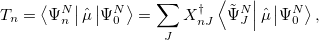
This also allows for the calculation of dipole transition moments via
 |
(6.53) |
as well as excited state properties via
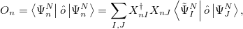 |
(6.54) |
where  is the property associated with operator
  .
.
Up to now, the exact  -electron ground state has been employed in the derivation of the ADC scheme, thereby resulting in exact excitation energies and exact excited state wave functions. Since the exact ground state is usually not known, a suitable approximation must be used in the derivation of the ISR equations. An obvious choice is the th order Møller-Plesset ground state yielding the th order approximation of the ADC scheme. The appropriate ADC equations have been derived in detail up to third order in Refs. Trofimov:1995,Trofimov:1999,Trofimov:2002. Due to the dependency on the Møller-Plesset ground state the th order ADC scheme should only be applied to molecular systems whose ground state is well described by the respective MP() method.
As in Møller-Plesset perturbation theory, the first ADC scheme which goes beyond the non-correlated wave function methods in Section 6.2 is ADC(2). ADC(2) is available in a strict and an extended variant which are usually referred to as ADC(2)-s and ADC(2)-x, respectively. The strict variant ADC(2)-s scales with the 5th power of the basis set. The quality of ADC(2)-s excitation energies and corresponding excited states is comparable to the quality of those obtained with CIS(D) (Section 6.6) or CC2. More precisely, excited states with mostly single excitation character are well-described by ADC(2)-s, while excited states with double excitation character are usually found to be too high in energy. The ADC(2)-x variant which scales as the sixth power of the basis set improves the treatment of doubly excited states, but at the cost of introducing an imbalance between singly and doubly excited states. As result, the excitation energies of doubly excited states are substantially decreased in ADC(2)-x relative to the states possessing mostly single excitation character with the excitation energies of both types of states exhibiting relatively large errors. Still, ADC(2)-x calculations can be used as a diagnostic tool for the importance doubly excited states in the low-energy region of the spectrum by comparing to ADC(2)-s results. A significantly better description of both singly and doubly excited states is provided by the third order ADC scheme ADC(3). The accuracy of excitation energies obtained with ADC(3) is almost comparable to CC3, but at computational costs that scale with the sixth power of the basis set only [425].
6.8.2 Resolution of the Identity ADC Methods
Similar to MP2 and CIS(D), the ADC equations can be reformulated using the resolution-of-the-identity (RI) approximation. This significantly reduces the cost of the integral transformation and the storage requirements. Although it does not change the overall computational scaling of  for ADC(2)-s or
  for ADC(2)-x with the system size, employing the RI approximation will result in computational speed-up of calculations of larger systems.
The RI approximation can be used with all available ADC methods. It is invoked as soon as an auxiliary basis set is specified using AUX_BASIS.
6.8.3 Spin Opposite Scaling ADC(2) Models
The spin-opposite scaling (SOS) approach originates from MP2 where it was realized that the same spin contributions can be completely neglected, if the opposite spin components are scaled appropriately. In a similar way it is possible to simplify the second order ADC equations by neglecting the same spin contributions in the ADC matrix, while the opposite-spin contributions are scaled with appropriate semi-empirical parameters. [434, 435, 426]
Starting from the SOS-MP2 ground state the same scaling parameter  is introduced into the ADC equations to scale the
  amplitudes. This alone, however, does not result in any computational savings or substantial improvements of the ADC(2) results. In addition, the opposite spin components in the ph/2p2h and 2p2h/ph coupling blocks have to be scaled using a second parameter
  to obtain a useful SOS-ADC(2)-s model. With this model the optimal value of the parameter has been found to be 1.17 for the calculation of singlet excited states.[435]
To extend the SOS approximation to the ADC(2)-x method yet another scaling parameter  for the opposite spin components of the off-diagonal elements in the 2p2h/2p2h block has to be introduced. Here, the optimal values of the scaling parameters have been determined as
  and
and  keeping
  unchanged.[426]
The spin-opposite scaling models can be invoked by setting METHOD to either SOSADC(2) or SOSADC(2)-x. By default, the scaling parameters are chosen as the optimal values reported above, i.e. and  for ADC(2)-s and , , and for ADC(2)-x. However, it is possible to adjust any of the three parameters by setting ADC_C_T, ADC_C_C, or ADC_C_X, respectively.
6.8.4 Core-Excitation ADC Methods
Core-excited electronic states are located in the high energy X-ray region of the spectrum. Thus, to compute core-excited states using standard diagonalization procedures, which usually solve for the energetically lowest-lying excited states first, requires the calculation of a multitude of excited states. This is computationally very expensive and only feasible for calculations on very small molecules and small basis sets.
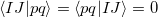
The core-valence separation (CVS) approximation solves the problem by neglecting the couplings between core and valence excited states a priori. [436, 437] Thereby, the ADC matrix acquires a certain block structure which allows to solve only for core-excited states. The application of the CVS approximation is justified, since core and valence excited states are energetically well separated and the coupling between both types of states is very small. To achieve the separation of core and valence excited states the CVS approximation forces the following types of two-electron integrals to zero
 |
|||
 |
(6.55) | ||
 |
where capital letters  refer to core orbitals while lower-case letters
  denote non-core occupied or virtual orbitals.
The core-valence approximation is currently available of ADC models up to second order (including the extended variant). [427, 428] It can be invoked by setting METHOD to the respective ADC model prefixed by CVS. Besides the general ADC related keywords, two additional keywords in the $rem block are necessary to control CVS-ADC calculations:
ADC_CVS = TRUE switches on the CVS-ADC calculation
CC_REST_OCC = n controls the number of core orbitals included in the excitation space. The integer n corresponds to the n energetically lowest core orbitals.
Example: cytosine with the molecular formula C H
H N
N O includes one oxygen atom. To calculate O 1s core-excited states, CC_REST_OCC has to be set to 1, because the 1s orbital of oxygen is the energetically lowest. To obtain the N 1s core excitations, the integer has to be set to 4, because the 1s orbital of the oxygen atom is included as well, since it is energetically below the three 1s orbitals of the nitrogen atoms. Accordingly, to simulate the C 1s XAS spectrum of cytosine, CC_REST_OCC must be set to 8.
To obtain the best agreement with experimental data, one should use the CVS-ADC(2)-x method in combination with at least a diffuse triple- basis set. [427, 428, 438]
6.8.5 Spin-Flip ADC Methods
The spin-flip (SF) method [400, 353, 407, 439] is used for molecular systems with few-reference wave functions like diradicals, bond-breaking, rotations around single bonds, and conical intersections. Starting from a triplet ( ) ground state reference a spin-flip excitation operator
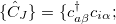

 is introduced, which flipped the spin of one electron while singlet and (
 ) triplet excited target states are yielded. The spin-flip method is implemented for the ADC(2) (strict and extended) and the ADC(3) methods. [439] Note that high-spin () triplet states can be calculated with the SF-ADC method as well using a closed-shell singlet reference state. The number of spin-flip states that shall be calculated is controlled with the $rem variable SF_STATES.
6.8.6 Properties and Visualization
The calculation of excited states using the ADCMAN module yields by default the usual excitation energies and the excitation amplitudes, as well as the transition dipole moments, oscillator strengths, and the norm of the doubles part of the amplitudes (if applicable). In addition, the calculation of excited state properties, like dipole moments, and transition properties between excited states can be requested by setting the $rem variables ADC_PROP_ES and ADC_PROP_ES2ES, respectively. Resonant two-photon absorption cross-sections of the excited states can be computed as well, using either sum-over-states expressions or the matrix inversion technique. The calculation via sum-over-state expressions is automatically activated, if ADC_PROP_ES2ES is set. The accuracy of the results, however, strongly depends on the number of states which are included in the summation, i.e. the number of states computed. At least, 20-30 excited states (per irreducible representation) are required to yield useful results for the two-photon absorption cross-sections. Alternatively, the resonant two-photon absorption cross-sections can be calculated by setting ADC_PROP_TPA to TRUE. In this case, the computation of a large number of excited states is avoided and there is no dependence on the number of excited states. Instead, an additional linear matrix equation has to be solved for every excited state for which the two-photon absorption cross-section is computed. Thus, the obtained resonant two-photon absorption cross-sections are usually more reliable.
Furthermore, the ADCMAN module allows for the detailed analysis of the excited states and export of various types of excited state related orbitals and densities. This can be activated by setting the keyword STATE_ANALYSIS. Details on the available analyses and export options can be found in section 10.2.7.
6.8.7 Vertical Excitation Energies in Solution with PCM Non-Equilibrium Corrections
Vertical excitation energies in solution with PCM non-equilibrium corrections can be computed at all orders (1, 2s, 2x, 3) of ADC for the polarization propagator including also the respective SCS and SOS variants. In principle, the calculation of PCM corrections for SF-ADC is also possible, one has to mind however, that there exists some ambiguity in the definition of the reference state, which is not yet automatically resolved. To perform a PCM-ADC calculation, one has to invoke the PCM (SOLVENT_METHOD to PCM in the $rem block) and specify the solvent parameters, i.e. the dielectric constant  and the squared refractive index
  (DIELECTRIC and DIELECTRIC_INFI in the $solvent block). If nothing is given, the parameters for water will be used by default. For a detailed description of the PCM, the user is referred to section 11.2.2 and 11.2.3. We recommend the use of the formally exact and slightly more expensive integral-equation formalism (IEF)-PCM variant (THEORY to IEFPCM in the $pcm block) instead of the approximate C-PCM and default parameters otherwise.
In a nutshell, an ADC/PCM calculation works as follows: A Hartree-Fock calculation with a PCM, i.e. a self-consistent reaction-field (SCRF) calculation is carried out and the final reaction field (essentially a set of point charges on the molecular surface) is separated according to the Franck-Condon principle into a slow, nuclear () and a fast, electronic () component. The resulting, polarized MOs are subjected to an normal ADC calculation which yields excited-state energies and densities. Eventually, while the slow component is kept frozen, the fast component of the reaction field and the respective interaction energy is recomputed for each excited-state density, thereby providing a first-order correction to the respective excitation energy. The described procedure corresponds to the perturbative, state-specific (ptSS) approach presented in Ref. [440]. A perturbative variant of the so-called linear response corrections (termed ptLR) is also available. In contrast to the ptSS approach, the ptLR corrections depend on the transition rather than the state (difference) densities. Although the ptLR corrections are always computed and printed, we do not recommend to use them with the correlated ADC variants (2 and higher), for which the ptSS approach is much better suited. The ptSS and ptLR approaches are also available for TDDFT as described in Section 11.2.2.3.
A drawback of the ptSS (also ptLR) approach as described above is the computation of the ground-state reaction-field (RF) at the HF level of theory. Since the interaction with the RF is contained in the MOs, a poor description of the densities and resulting properties at the HF level can translate into significant errors in the excitation energies computed with ADC. This is the case e.g. for nitroaromatics. To correct for this, we developed and implemented a perturbative density correction (PTD), which accounts for the differences between the HF and MP densities without additional computation cost. The PTD corrections are computed automatically if ADC(2) and/or ADC(3) is invoked and hence an MP density is computed. An empirically scaled variant of this correction termed PTD* is also available. See Ref. [440] for a detailed description of the formalism along with benchmarking and parametrization. Although the PTD correction also yields a (typically small) correction for the MP ground-state energy that is printed in the output, we recommend the use of the uncorrected energy. The reason being that only the latter is fully consistent with MP theory and in our experience also more accurate. Accordingly, the PTD ground-state correction is not included in the total excited state energies.
For the sake of traceability, the output obeys the following convention: Total energies of ground- and excited states always correspond to the pure eigenvalues of the respective wave functions, i.e. they do not include any perturbative ptLR, ptSS or PTD corrections. Specifically, the ADC total energy of an excited state is the sum of the HF energy, the MP correlation energy, and the zeroth-order excitation energy. Only in the excitation energies we include the respective ptSS/ptLR and PTD corrections as stated in the output. Depending on the order of ADC, the recommended excitation energy is given first (ptLR for ADC(1), ptSS(PTD) for ADC(2) and ADC(3)). Additionally, the uncorrected excitation energies as well as correction terms are also printed. An even more detailed output of all integrals contributing to the ptSS corrections like e.g. the sums of all polarization and interaction terms is if the PCM print level is increased (PCM_PRINT to 1 in the $rem block).
6.8.8 ADC Job Control
For an ADC calculation it is important to ensure that there are sufficient resources available for the necessary integral calculations and transformations. These resources are controlled using the $rem variables MEM_STATIC and MEM_TOTAL. The memory used by ADC is currently 95% of the difference MEM_TOTAL - MEM_STATIC.
An ADC calculation is requested by setting the $rem variable METHOD to the respective ADC variant. Furthermore, the number of excited states to be calculated has to be specified using one of the $rem variables EE_STATES, EE_SINGLETS, or EE_TRIPLETS. The former variable should be used for open-shell or unrestricted closed-shell calculations, while the latter two variables are intended for restricted closed-shell calculations. Even though not recommended, it is possible to use EE_STATES in a restricted calculation which translates into EE_SINGLETS, if neither EE_SINGLETS nor EE_TRIPLETS is set. Similarly, the use EE_SINGLETS in an unrestricted calculation will translate into EE_STATES, if the latter is not set as well.
All $rem variables to set the number of excited states accept either an integer number or a vector of integer numbers. A single number specifies that the same number of excited states are calculated for every irreducible representation the point group of the molecular system possesses (molecules without symmetry are treated as  symmetric). In contrast, a vector of numbers determines the number of states for each irreducible representation explicitly. Thus, the length of the vector always has to match the number of irreducible representations. Hereby, the excited states are labeled according to the irreducible representation of the electronic transition which might be different from the irreducible representation of the excited state wave function. Users can choose to calculate any molecule as symmetric by setting CC_SYMMETRY to FALSE.
METHOD
Controls the order in perturbation theory of ADC.
TYPE:
STRING
DEFAULT:
None
OPTIONS:
ADC(1)
Perform ADC(1) calculation.
ADC(2)
Perform ADC(2)-s calculation.
ADC(2)-x
Perform ADC(2)-x calculation.
ADC(3)
Perform ADC(3) calculation.
SOS-ADC(2)
Perform spin-opposite scaled ADC(2)-s calculation.
SOS-ADC(2)-x
Perform spin-opposite scaled ADC(2)-x calculation.
CVS-ADC(1)
Perform ADC(1) calculation of core excitations.
CVS-ADC(2)
Perform ADC(2)-s calculation of core excitations.
CVS-ADC(2)-x
Perform ADC(2)-x calculation of core excitations.
RECOMMENDATION:
None
EE_STATES
Controls the number of excited states to calculate.
TYPE:
INTEGER
DEFAULT:
0
Do not perform an ADC calculation
OPTIONS:

Number of states to calculate for each irrep or
![$[n_1, n_2, ...]$](images/img-0905.png)
Compute
states for the first irrep,
states for the second irrep, ...
RECOMMENDATION:
Use this variable to define the number of excited states in case of unrestricted or open-shell calculations. In restricted calculations it can also be used, if neither EE_SINGLETS nor EE_TRIPLETS is given. Then, it has the same effect as setting EE_SINGLETS.
EE_SINGLETS
Controls the number of singlet excited states to calculate.
TYPE:
INTEGER
DEFAULT:
0
Do not perform an ADC calculation of singlet excited states
OPTIONS:
Number of singlet states to calculate for each irrep or
Compute
RECOMMENDATION:
Use this variable to define the number of excited states in case of restricted calculations of singlet states. In unrestricted calculations it can also be used, if EE_STATES not set. Then, it has the same effect as setting EE_STATES.
EE_TRIPLETS
Controls the number of triplet excited states to calculate.
TYPE:
INTEGER/INTEGER ARRAY
DEFAULT:
0
Do not perform an ADC calculation of triplet excited states
OPTIONS:
Number of triplet states to calculate for each irrep or
Compute
RECOMMENDATION:
Use this variable to define the number of excited states in case of restricted calculations of triplet states.
CC_SYMMETRY
Activates point-group symmetry in the ADC calculation.
TYPE:
LOGICAL
DEFAULT:
TRUE
If the system possesses any point-group symmetry.
OPTIONS:
TRUE
Employ point-group symmetry
FALSE
Do not use point-group symmetry
RECOMMENDATION:
None
ADC_PROP_ES
Controls the calculation of excited state properties (currently only dipole moments).
TYPE:
LOGICAL
DEFAULT:
FALSE
OPTIONS:
TRUE
Calculate excited state properties.
FALSE
Do not compute state properties.
RECOMMENDATION:
Set to TRUE, if properties are required.
ADC_PROP_ES2ES
Controls the calculation of transition properties between excited states (currently only transition dipole moments and oscillator strengths), as well as the computation of two-photon absorption cross-sections of excited states using the sum-over-states expression.
TYPE:
LOGICAL
DEFAULT:
FALSE
OPTIONS:
TRUE
Calculate state-to-state transition properties.
FALSE
Do not compute transition properties between excited states.
RECOMMENDATION:
Set to TRUE, if state-to-state properties or sum-over-states two-photon absorption cross-sections are required.
ADC_PROP_TPA
Controls the calculation of two-photon absorption cross-sections of excited states using matrix inversion techniques.
TYPE:
LOGICAL
DEFAULT:
FALSE
OPTIONS:
TRUE
Calculate two-photon absorption cross-sections.
FALSE
Do not compute two-photon absorption cross-sections.
RECOMMENDATION:
Set to TRUE, if to obtain two-photon absorption cross-sections.
STATE_ANALYSIS
Controls the analysis and export of excited state densities and orbitals (see 10.2.7 for details).
TYPE:
LOGICAL
DEFAULT:
FALSE
OPTIONS:
TRUE
Perform excited state analyses.
FALSE
No excited state analyses or export will be performed.
RECOMMENDATION:
Set to TRUE, if detailed analysis of the excited states is required or if density or orbital plots are needed.
ADC_C_T
Set the spin-opposite scaling parameter
.
TYPE:
INTEGER
DEFAULT:
1300
Optimized value
.
OPTIONS:
Corresponding to

RECOMMENDATION:
Use the default.
ADC_C_C
Set the spin-opposite scaling parameter
TYPE:
INTEGER
DEFAULT:
1170
Optimized value
1000
OPTIONS:
Corresponding to
RECOMMENDATION:
Use the default.
ADC_C_X
Set the spin-opposite scaling parameter
TYPE:
INTEGER
DEFAULT:
1300
Optimized value
for ADC(2)-x.
OPTIONS:
Corresponding to
RECOMMENDATION:
Use the default.
ADC_NGUESS_SINGLES
Controls the number of excited state guess vectors which are single excitations. If the number of requested excited states exceeds the total number of guess vectors (singles and doubles), this parameter is automatically adjusted, so that the number of guess vectors matches the number of requested excited states.
TYPE:
INTEGER
DEFAULT:
Equals to the number of excited states requested.
OPTIONS:
User-defined integer.
RECOMMENDATION:
ADC_NGUESS_DOUBLES
Controls the number of excited state guess vectors which are double excitations.
TYPE:
INTEGER
DEFAULT:
0
OPTIONS:
User-defined integer.
RECOMMENDATION:
ADC_DO_DIIS
Activates the use of the DIIS algorithm for the calculation of ADC(2) excited states.
TYPE:
LOGICAL
DEFAULT:
FALSE
OPTIONS:
TRUE
Use DIIS algorithm.
FALSE
Do diagonalization using Davidson algorithm.
RECOMMENDATION:
None.
ADC_DIIS_START
Controls the iteration step at which DIIS is turned on.
TYPE:
INTEGER
DEFAULT:
1
OPTIONS:
User-defined integer.
RECOMMENDATION:
Set to a large number to switch off DIIS steps.
ADC_DIIS_SIZE
Controls the size of the DIIS subspace.
TYPE:
INTEGER
DEFAULT:
7
OPTIONS:
User-defined integer
RECOMMENDATION:
None
ADC_DIIS_MAXITER
Controls the maximum number of DIIS iterations.
TYPE:
INTEGER
DEFAULT:
50
OPTIONS:
User-defined integer.
RECOMMENDATION:
Increase in case of slow convergence.
ADC_DIIS_ECONV
Controls the convergence criterion for the excited state energy during DIIS.
TYPE:
INTEGER
DEFAULT:
6
Corresponding to

OPTIONS:
Corresponding to

RECOMMENDATION:
None
ADC_DIIS_RCONV
Convergence criterion for the residual vector norm of the excited state during DIIS.
TYPE:
INTEGER
DEFAULT:
6
Corresponding to
OPTIONS:
Corresponding to
RECOMMENDATION:
None
ADC_DAVIDSON_MAXSUBSPACE
Controls the maximum subspace size for the Davidson procedure.
TYPE:
INTEGER
DEFAULT:
the number of excited states to be calculated.
OPTIONS:
User-defined integer.
RECOMMENDATION:
Should be at least
the number of excited states to calculate. The larger the value the more disk space is required.
ADC_DAVIDSON_MAXITER
Controls the maximum number of iterations of the Davidson procedure.
TYPE:
INTEGER
DEFAULT:
60
OPTIONS:
Number of iterations
RECOMMENDATION:
Use the default unless convergence problems are encountered.
ADC_DAVIDSON_CONV
Controls the convergence criterion of the Davidson procedure.
TYPE:
INTEGER
DEFAULT:

Corresponding to
OPTIONS:

Corresponding to
RECOMMENDATION:
Use the default unless higher accuracy is required or convergence problems are encountered.
ADC_DAVIDSON_THRESH
Controls the threshold for the norm of expansion vectors to be added during the Davidson procedure.
TYPE:
INTEGER
DEFAULT:
Twice the value of ADC_DAVIDSON_CONV, but at maximum
.
OPTIONS:

Corresponding to
RECOMMENDATION:
Use the default unless convergence problems are encountered. The threshold value
ADC_PRINT
Controls the amount of printing during an ADC calculation.
TYPE:
INTEGER
DEFAULT:
1
Basic status information and results are printed.
OPTIONS:
0
Quiet: almost only results are printed.
1
Normal: basic status information and results are printed.
2
Debug: more status information, extended information on timings.
...
RECOMMENDATION:
Use the default.
ADC_CVS
Activates the use of the CVS approximation for the calculation of CVS-ADC core-excited states.
TYPE:
LOGICAL
DEFAULT:
FALSE
OPTIONS:
TRUE
Activates the CVS approximation.
FALSE
Do not compute core-excited states using the CVS approximation.
RECOMMENDATION:
Set to TRUE, if to obtain core-excited states for the simulation of X-ray absorption spectra. In the case of TRUE, the $rem variable CC_REST_OCC has to be defined as well.
CC_REST_OCC
Sets the number of restricted occupied orbitals including active core occupied orbitals.
TYPE:
INTEGER
DEFAULT:
0
OPTIONS:
Restrict
RECOMMENDATION:
Example: cytosine with the molecular formula C
SF_STATES
Controls the number of excited spin-flip states to calculate.
TYPE:
INTEGER
DEFAULT:
0
Do not perform a SF-ADC calculation
OPTIONS:
Number of states to calculate for each irrep or
Compute
RECOMMENDATION:
Use this variable to define the number of excited states in the case of a spin-flip calculation. SF-ADC is available for ADC(2)-s, ADC(2)-x and ADC(3).
6.8.9 Examples
Example 6.164 Q-Chem input for an ADC(2)-s calculation of singlet exited states of methane with D2 symmetry. In total six excited states are requested corresponding to four (two) electronic transitions with irreducible representation  (
( ).
).
$molecule
0 1
C
H   1 r0
H   1 r0   2  d0
H   1 r0   2  d0   3  d1
H   1 r0   2  d0   4  d1

r0 = 1.085
d0 = 109.4712206
d1 = 120.0
$end

$rem
jobtype             sp
method              adc(2)
basis               6-31g(d,p)
mem_total           4000
mem_static          100
ee_singlets         [0,4,2,0]
$end
Example 6.165 Q-Chem input for an unrestricted RI-ADC(2)-s calculation with symmetry using DIIS. In addition, excited state properties and state-to-state properties are computed.
$molecule
0 2
C    0.0    0.0   -0.630969
N    0.0    0.0    0.540831
$end

$rem
jobtype             sp
method              adc(2)
basis               aug-cc-pVDZ
aux_basis		rimp2-aug-cc-pVDZ
mem_total           4000
mem_static          100
cc_symmetry         false
ee_states           6
adc_do_diis         true
adc_prop_es         true
adc_prop_es2es      true
adc_prop_tpa        true
$end
Example 6.166 Q-Chem input for a restricted CVS-ADC(2)-x calculation with symmetry using 4 parallel CPU cores. In this case, the 10 lowest nitrogen K-shell singlet excitations are computed.
$molecule
0 1
C    -5.17920    2.21618    0.01098
C    -3.85603    2.79078    0.05749
N    -2.74877    2.08372    0.05569
C    -5.23385    0.85443   -0.04040
C    -2.78766    0.70838    0.01226
N    -4.08565    0.13372   -0.03930
N    -3.73433    4.14564    0.16144
O    -1.81716   -0.02560    0.00909
H    -4.50497    4.74117   -0.12037
H    -2.79158    4.50980    0.04490
H    -4.10443   -0.88340   -0.07575
H    -6.08637    2.82445    0.02474
H    -6.17341    0.29221   -0.07941
$end

$rem
jobtype                     sp
method                      cvs-adc(2)-x
ee_singlets                 10
adc_davidson_maxsubspace    60
mem_total                   10000
mem_static                  1000
Threads                     4
cc_symmetry                 false
basis                       6-31G*
ADC_Davidson_thresh         8
Symmetry                    false
ADC_DAVIDSON_MAXITER        900
ADC_CVS                     true
cc_rest_occ                 4
$end
Example 6.167 Q-Chem input for a restricted SF-ADC(2)-s calculation of the first three spin-flip target states of cyclobutadiene without point group symmetry.
$molecule
0 3
 C     0.000000     0.000000     0.000000
 C     1.439000     0.000000     0.000000
 C     1.439000     0.000000     1.439000
 C     0.000000     0.000000     1.439000
 H    -0.758726     0.000000    -0.758726
 H     2.197726     0.000000    -0.758726
 H     2.197726     0.000000     2.197726
 H    -0.758726     0.000000     2.197726
$end

$rem
jobtype         sp
method          adc(2)
mem_total       15000
mem_static      1000
cc_symmetry     false
basis           3-21G
sf_states       3
$end
Example 6.168 Q-Chem input for a restricted ADC(2)-x calculation of water with  symmetry. Four singlet A" excited states and two triplet A’ excited states are requested. For the first two states (1
 A" and 1
 A’) the transition densities as well as the attachment and detachment densities are exported into cube files.
$molecule
0 1
O   0.000   0.000   0.000
H   0.000   0.000   0.950
H   0.896   0.000  -0.317
$end

$rem
jobtype             sp
method              adc(2)-x
basis               6-31g(d,p)
threads             2
mem_total           3000
mem_static          100
ee_singlets         [0,4]
ee_triplets         [2,0]
adc_prop_es         true

make_cube_files     true
$end

$plots
Plot transition and a/d densities
40 -3.0 3.0
40 -3.0 3.0
40 -3.0 3.0
0 0 2 2
1 2
1 2
$end
Example 6.169 Q-Chem input for a restricted ADC(2)-s calculation of N,N-dimethylnitroaniline in diethylether. Five singlet excited states are requested. PCM settings are all default values except THEORY, which is set to IEFPCM instead of the default CPCM.
$rem
threads                4
method                 adc(2)
basis                  3-21G
mem_total              32000
mem_static             2000
adc_prop_es            true
adc_print              1
EE_SINGLETS            5
adc_davidson_maxiter   100
pcm_print              1       !increase print level
solvent_method         pcm     !invokes PCM solvent model
$end

$pcm
StateSpecific           Perturb !default for ADC/PCM
ChargeSeparation        Marcus  !default
theory                  IEFPCM  !default is CPCM, IEFPCM is more accurate
method                  ISWIG
Solver                  Inversion
Radii                   Bondi
vdwScale                1.20
$end

$solvent
dielectric              4.34  !epsilon of Et2O
dielectric_infi         1.829 !n_square of Et2O
$end

$molecule
0 1
  C   -4.263068      2.512843      0.025391
  C   -5.030982      1.361365      0.007383
  C   -4.428196      0.076338     -0.021323
  C   -3.009941      0.019036     -0.030206
  C   -2.243560      1.171441     -0.011984
  C   -2.871710      2.416638      0.015684
  H   -4.740854      3.480454      0.047090
  H   -2.502361     -0.932570     -0.052168
  H   -1.166655      1.104642     -0.020011
  H   -6.104933      1.461766      0.015870
  N   -5.178541     -1.053870     -0.039597
  C   -6.632186     -0.969550     -0.034925
  H   -6.998203     -0.462970      0.860349
  H   -7.038179     -1.975370     -0.051945
  H   -7.001616     -0.431420     -0.910237
  C   -4.531894     -2.358860     -0.066222
  H   -3.912683     -2.476270     -0.957890
  H   -5.298508     -3.126680     -0.075403
  H   -3.902757     -2.507480      0.813678
  N   -2.070815      3.621238      0.033076
  O   -0.842606      3.510489      0.025476
  O   -2.648404      4.710370      0.054545
$end