4.10 Methods Based on “Constrained” DFT
4.10.1 Theory
Under certain circumstances it is desirable to apply constraints to the electron density during an SCF calculation. For example, in a transition metal complex it may be desirable to constrain the net spin density on a particular metal atom to integrate to a value consistent with the  value expected from ligand field theory. Similarly, in a donor–acceptor complex one might be interested in constraining the total density on the acceptor group so that the formal charge on the acceptor is either neutral or negatively charged, depending as the molecule is in its neutral or its charge-transfer state. In these situations, one is interested in controlling the average value of some observable,
  , to take on a given value,
  :
:
 |
(4.100) |
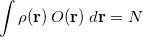
There are of course many states that satisfy such a constraint, but in practice one is usually looking for the lowest energy such state. To solve the resulting constrained minimization problem, one introduces a Lagrange multiplier,  , and solves for the stationary point of
![\begin{equation} V[\rho , V] = E[\rho ] - V\left(\int \rho (\mathbf{r}) \, O(\mathbf{r}) \; d\mathbf{r} - N \right) \end{equation}](images/img-0438.png) |
(4.101) |
where ![$E[\rho ]$](images/img-0439.png) is the energy of the system described using density functional theory (DFT). At convergence, the functional
is the energy of the system described using density functional theory (DFT). At convergence, the functional  gives the density,
  , that satisfies the constraint exactly (i.e., it has exactly the prescribed number of electrons on the acceptor or spins on the metal center) but has the lowest energy possible. The resulting self-consistent procedure can be efficiently solved by ensuring at every SCF step the constraint is satisfied exactly. The Q-Chem implementation of these equations closely parallels those in Ref. Wu:2005.
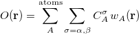
The first step in any constrained DFT calculation is the specification of the constraint operator, . Within Q-Chem, the user is free to specify any constraint operator that consists of a linear combination of the Becke’s atomic partitioning functions [142]:
 |
(4.102) |
Here the summation runs over the atoms in the system and over electron spins. The weight function  is designed to be
  near the nucleus of atom
  and rapidly fall to zero near the nucleus of any other atom in the system [142]. The user-specified coefficients
  are input using a $cdft input section having the following format.
$cdft
CONSTRAINT_VALUE_X
COEFFICIENT1_X       FIRST_ATOM1_X       LAST_ATOM1_X    TYPE1_X
COEFFICIENT2_X       FIRST_ATOM2_X       LAST_ATOM2_X    TYPE2_X
...
CONSTRAINT_VALUE_Y
COEFFICIENT1_Y       FIRST_ATOM1_Y       LAST_ATOM1_Y    TYPE1_Y
COEFFICIENT2_Y       FIRST_ATOM2_Y       LAST_ATOM2_Y    TYPE2_Y
...
...
$end
Here, each CONSTRAINT_VALUE is a real number that specifies the desired average value () of the ensuing linear combination of atomic partition functions. Each COEFFICIENT specifies the coefficient of a partition function or group of partition functions in the constraint operator  . For each coefficient, all the atoms between the integers FIRST_ATOM and LAST_ATOM contribute with the specified weight in the constraint operator. Finally, TYPE specifies the type of constraint being applied—either “CHARGE” or “SPIN”. For a CHARGE constraint the spin up and spin down densities contribute equally (
 ) yielding the total number of electrons on the atom A. For a SPIN constraint, the spin up and spin down densities contribute with opposite sign (
 ) resulting in a measure of the net spin on the atom A. Each separate CONSTRAINT_VALUE creates a new operator whose average is to be constrained—for instance, the example above includes several independent constraints:
  . Q-Chem can handle an arbitrary number of constraints and will minimize the energy subject to all of these constraints simultaneously.
If an atom is not included in a particular operator, then the coefficient of that atoms partition function is set to zero for that operator. The TYPE specification is optional, and the default is to perform a charge constraint. Further, note that any charge constraint is on the net atomic charge. That is, the constraint is on the difference between the average number of electrons on the atom and the nuclear charge. Thus, to constrain CO to be negative, the constraint value would be 1 and not 15.
Note: Charge constraint in $cdft specifies the number of excess electrons on a fragment, not the total charge, i.e., the value 1.0 means charge  , whereas charge constraint of
  1.0 corresponds to the total
  1 charge.
The choice of which atoms to include in different constraint regions is left entirely to the user and in practice must be based somewhat on chemical intuition. Thus, for example, in an electron transfer reaction the user must specify which atoms are in the “donor” and which are in the “acceptor”. In practice, the most stable choice is typically to make the constrained region as large as physically possible. Thus, for the example of electron transfer again, it is best to assign every atom in the molecule to one or the other group (donor or acceptor), recognizing that it makes no sense to assign any atoms to both groups. On the other end of the spectrum, constraining the formal charge on a single atom is highly discouraged. The problem is that while our chemical intuition tells us that the lithium atom in LiF should have a formal charge of +1, in practice the quantum mechanical charge is much closer to +0.5 than +1. Only when the fragments are far enough apart do our intuitive pictures of formal charge actually become quantitative.
Note that the atomic populations that Q-Chem prints out are Mulliken populations, not the Becke weight populations. As a result, the printed populations will not generally add up to the specified constrained values, even though the constraint is exactly satisfied. You can print Becke populations to confirm that the computed states have the desired charge/spin character.
Finally, we note that SCF convergence is typically more challenging in constrained DFT calculations as compared to their unconstrained counterparts. This effect arises because applying the constraint typically leads to a broken symmetry, diradical-like state. As SCF convergence for these cases is known to be difficult even for unconstrained states, it is perhaps not surprising that there are additional convergence difficulties in this case. See Section 4.6 on SCF convergence algorithms for ideas on how to improve convergence for constrained calculations. Also, CDFT is more sensitive to grid size than ground-state DFT, so sometimes increasing the integration grid to (50,194) or (75, 302), instead of the default SG-1 grid, improves the convergence.
Note: (i) To improve convergence, use the fewest possible constraints. For example, if your system consists of two fragments, specify the constrains for one of them only. The overall charge and multiplicity will force the “unconstrained” fragment to attain the right charge and multiplicity.
(ii) The direct minimization methods are not available for constrained calculations. Hence, some combination of DIIS and RCA must be used to obtain convergence. Further, it is often necessary to break symmetry in the initial guess (using SCF_GUESS_MIX) to ensure that the lowest energy solution is obtained.
Analytic gradients are available for constrained DFT calculations [250]. Second derivatives are only available by finite difference of analytic gradients. For details on how to apply constrained DFT to compute magnetic exchange couplings, see Ref. Wu:2006b. For details on using constrained DFT to compute electron transfer parameters, see Ref. Wu:2006c.
4.10.2 CDFT Job Control and Examples
A CDFT calculation is requested by setting CDFT = TRUE in the $rem section, as as by specifying a $cdft input section as described above. Additional job control variables are described below.
CDFT
Initiates a constrained DFT calculation
TYPE:
LOGICAL
DEFAULT:
FALSE
OPTIONS:
TRUE
Perform a Constrained DFT Calculation
FALSE
No Density Constraint
RECOMMENDATION:
Set to TRUE if a Constrained DFT calculation is desired.
CDFT_POSTDIIS
Controls whether the constraint is enforced after DIIS extrapolation.
TYPE:
LOGICAL
DEFAULT:
TRUE
OPTIONS:
TRUE
Enforce constraint after DIIS
FALSE
Do not enforce constraint after DIIS
RECOMMENDATION:
Use the default unless convergence problems arise, in which case it may be beneficial to experiment with setting CDFT_POSTDIIS to FALSE. With this option set to TRUE, energies should be variational after the first iteration.
CDFT_PREDIIS
Controls whether the constraint is enforced before DIIS extrapolation.
TYPE:
LOGICAL
DEFAULT:
FALSE
OPTIONS:
TRUE
Enforce constraint before DIIS
FALSE
Do not enforce constraint before DIIS
RECOMMENDATION:
Use the default unless convergence problems arise, in which case it may be beneficial to experiment with setting CDFT_PREDIIS to TRUE. Note that it is possible to enforce the constraint both before and after DIIS by setting both CDFT_PREDIIS and CDFT_POSTDIIS to TRUE.
CDFT_THRESH
Threshold that determines how tightly the constraint must be satisfied.
TYPE:
INTEGER
DEFAULT:
5
OPTIONS:
N
Constraint is satisfied to within
.
RECOMMENDATION:
Use the default unless problems occur.
CDFT_CRASHONFAIL
Whether the calculation should crash or not if the constraint iterations do not converge.
TYPE:
LOGICAL
DEFAULT:
TRUE
OPTIONS:
TRUE
Crash if constraint iterations do not converge.
FALSE
Do not crash.
RECOMMENDATION:
Use the default.
CDFT_BECKE_POP
Whether the calculation should print the Becke atomic charges at convergence
TYPE:
LOGICAL
DEFAULT:
TRUE
OPTIONS:
TRUE
Print Populations
FALSE
Do not print them
RECOMMENDATION:
Use the default. Note that the Mulliken populations printed at the end of an SCF run will not typically add up to the prescribed constraint value. Only the Becke populations are guaranteed to satisfy the user-specified constraints.
Example 4.64 Charge separation on FAAQ
$molecule
0 1
 C     -0.64570736     1.37641945    -0.59867467
 C      0.64047568     1.86965826    -0.50242683
 C      1.73542663     1.01169939    -0.26307089
 C      1.48977850    -0.39245666    -0.15200261
 C      0.17444585    -0.86520769    -0.27283957
 C     -0.91002699    -0.02021483    -0.46970395
 C      3.07770780     1.57576311    -0.14660056
 C      2.57383948    -1.35303134     0.09158744
 C      3.93006075    -0.78485926     0.20164558
 C      4.16915637     0.61104948     0.08827557
 C      5.48914671     1.09087541     0.20409492
 H      5.64130588     2.16192921     0.11315072
 C      6.54456054     0.22164774     0.42486947
 C      6.30689287    -1.16262761     0.53756193
 C      5.01647654    -1.65329553     0.42726664
 H     -1.45105590     2.07404495    -0.83914389
 H      0.85607395     2.92830339    -0.61585218
 H      0.02533661    -1.93964850    -0.19096085
 H      7.55839768     0.60647405     0.51134530
 H      7.13705743    -1.84392666     0.71043613
 H      4.80090178    -2.71421422     0.50926027
 O      2.35714021    -2.57891545     0.20103599
 O      3.29128460     2.80678842    -0.23826460
 C     -2.29106231    -0.63197545    -0.53957285
 O     -2.55084900    -1.72562847    -0.95628300
 N     -3.24209015     0.26680616     0.03199109
 H     -2.81592456     1.08883943     0.45966550
 C     -4.58411403     0.11982669     0.15424004
 C     -5.28753695     1.14948617     0.86238753
 C     -5.30144592    -0.99369577    -0.39253179
 C     -6.65078185     1.06387425     1.01814801
 H     -4.73058059     1.98862544     1.26980479
 C     -6.66791492    -1.05241167    -0.21955088
 H     -4.76132422    -1.76584307    -0.92242502
 C     -7.35245187    -0.03698606     0.47966072
 H     -7.18656323     1.84034269     1.55377875
 H     -7.22179827    -1.89092743    -0.62856041
 H     -8.42896369    -0.10082875     0.60432214
$end

$rem
JOBTYPE         FORCE
METHOD          B3LYP
BASIS           6-31G*
SCF_PRINT       TRUE
CDFT            TRUE
$end

$cdft
2
 1 1  25
-1 26 38
$end
Example 4.65 Cu2-Ox High Spin
$molecule
2 3
 Cu      1.4674     1.6370     1.5762
 O       1.7093     0.0850     0.3825
 O      -0.5891     1.3402     0.9352
 C       0.6487    -0.3651    -0.1716
 N       1.2005     3.2680     2.7240
 N       3.0386     2.6879     0.6981
 N       1.3597     0.4651     3.4308
 H       2.1491    -0.1464     3.4851
 H       0.5184    -0.0755     3.4352
 H       1.3626     1.0836     4.2166
 H       1.9316     3.3202     3.4043
 H       0.3168     3.2079     3.1883
 H       1.2204     4.0865     2.1499
 H       3.8375     2.6565     1.2987
 H       3.2668     2.2722    -0.1823
 H       2.7652     3.6394     0.5565
 Cu     -1.4674    -1.6370    -1.5762
 O      -1.7093    -0.0850    -0.3825
 O       0.5891    -1.3402    -0.9352
 C      -0.6487     0.3651     0.1716
 N      -1.2005    -3.2680    -2.7240
 N      -3.0386    -2.6879    -0.6981
 N      -1.3597    -0.4651    -3.4308
 H      -2.6704    -3.4097    -0.1120
 H      -3.6070    -3.0961    -1.4124
 H      -3.5921    -2.0622    -0.1485
 H      -0.3622    -3.1653    -3.2595
 H      -1.9799    -3.3721    -3.3417
 H      -1.1266    -4.0773    -2.1412
 H      -0.5359     0.1017    -3.4196
 H      -2.1667     0.1211    -3.5020
 H      -1.3275    -1.0845    -4.2152
$end

$rem
JOBTYPE         SP
METHOD          B3LYP
BASIS           6-31G*
SCF_PRINT       TRUE
CDFT            TRUE
$end

$cdft
2
 1 1   3  s
-1 17 19  s
$end
4.10.3 Configuration Interaction with Constrained DFT (CDFT-CI)
There are some situations in which a system is not well-described by a DFT calculation on a single configuration. For example, transition states are known to be poorly described by most functionals, with the computed barrier being too low. We can, in particular, identify homolytic dissociation of diatomic species as situations where static correlation becomes extremely important. Existing DFT functionals have proved to be very effective in capturing dynamic correlation, but frequently exhibit difficulties in the presence of strong static correlation. Configuration Interaction, well known in wave function methods, is a multireference method that is quite well-suited for capturing static correlation; the CDFT-CI technique allows for CI calculations on top of DFT calculations, harnessing both static and dynamic correlation methods.
Constrained DFT is used to compute densities (and Kohn-Sham wave functions) for two or more diabatic-like states; these states are then used to build a CI matrix. Diagonalizing this matrix yields energies for the ground and excited states within the configuration space. The coefficients of the initial diabatic states are printed, to show the characteristics of the resultant states.
Since DFT only gives converged densities, not actual wave functions, computing the off-diagonal coupling elements  is not completely straightforward, as the physical meaning of the Kohn-Sham wave function is not entirely clear. We can, however, perform the following manipulation [253]:
![$\displaystyle \begin{aligned} H_{12} & = \frac{1}{2}\Bigl [\langle 1|H+V_{C_1}\omega ^{}_{C_1}-V_{C1}\omega ^{}_{C_1} |2\rangle + \langle 1|H+V_{C_2}\omega ^{}_{C_2}-V_{C_2}\omega ^{}_{C_2}|2\rangle \Bigr ]\\ & =\frac{1}{2}\Bigl [\left(E_1+V_{C_1}N_{C_1}+E_2+V_{C_2}N_{C_2}\right) \langle 1|2\rangle -V_{C_1}\langle 1|\omega ^{}_{C_1}|2\rangle -V_{C_2}\langle 1|\omega ^{}_{C_2}|2\rangle \Bigr ] \end{aligned} $](images/img-0452.png) |
(4.103) |
where the converged states  are assumed to be the ground state of
  with eigenvalue
  ). This manipulation eliminates the two-electron integrals from the expression, and experience has shown that the use of Slater determinants of Kohn-Sham orbitals is a reasonable approximation for the quantities
  and
and  .
.
Note that since these constrained states are eigenfunctions of different Hamiltonians (due to different constraining potentials), they are not orthogonal states, and we must set up our CI matrix as a generalized eigenvalue problem. Symmetric orthogonalization is used by default, though the overlap matrix and Hamiltonian in non-orthogonal basis are also printed at higher print levels so that other orthogonalization schemes can be used after-the-fact. In a limited number of cases, it is possible to find an orthogonal basis for the CDFT-CI Hamiltonian, where a physical interpretation can be assigned to the orthogonal states. In such cases, the matrix representation of the Becke weight operator is diagonalized, and the (orthogonal) eigenstates can be characterized [254]. This matrix is printed as the “CDFT-CI Population Matrix” at increased print levels.
In order to perform a CDFT-CI calculation, the interacting states must be defined, which is accomplished using a $cdft input section in a fashion similar to the specification of CDFT states:
$cdft
STATE_1_CONSTRAINT_VALUE_X
COEFFICIENT1_X       FIRST_ATOM1_X       LAST_ATOM1_X    TYPE1_X
COEFFICIENT2_X       FIRST_ATOM2_X       LAST_ATOM2_X    TYPE2_X
...
STATE_1_CONSTRAINT_VALUE_Y
COEFFICIENT1_Y       FIRST_ATOM1_Y       LAST_ATOM1_Y    TYPE1_Y
COEFFICIENT2_Y       FIRST_ATOM2_Y       LAST_ATOM2_Y    TYPE2_Y
...
...
---
STATE_2_CONSTRAINT_VALUE_X
COEFFICIENT1_X       FIRST_ATOM1_X       LAST_ATOM1_X    TYPE1_X
COEFFICIENT2_X       FIRST_ATOM2_X       LAST_ATOM2_X    TYPE2_X
...
STATE_2_CONSTRAINT_VALUE_Y
COEFFICIENT1_Y       FIRST_ATOM1_Y       LAST_ATOM1_Y    TYPE1_Y
COEFFICIENT2_Y       FIRST_ATOM2_Y       LAST_ATOM2_Y    TYPE2_Y
...
...
...
$end
Each state is specified with the CONSTRAINT_VALUE and the corresponding weights on sets of atoms whose average value should be the constraint value. Different states are separated by a single line containing three or more dash characters.
If it is desired to use an unconstrained state as one of the interacting configurations, charge and spin constraints of zero may be applied to the atom range from 0 to 0.
Note: It is mandatory to specify a spin constraint corresponding to every charge constraint (and it must be immediately following that charge constraint in the input deck), for reasons described below.
In addition to the $cdft input section of the input file, a CDFT-CI calculation must also set the CDFTCI flag to TRUE for the calculation to run. Note, however, that the CDFT flag is used internally by CDFT-CI, and should not be set in the input deck. The variable CDFTCI_PRINT may also be set manually to control the level of output. The default is 0, which will print the energies and weights (in the diabatic basis) of the CDFT-CI states. Setting it to 1 or above will also print the CDFT-CI overlap matrix, the CDFT-CI Hamiltonian matrix before the change of basis, and the CDFT-CI Population matrix. Setting it to 2 or above will also print the eigenvectors and eigenvalues of the CDFT-CI Population matrix. Setting it to 3 will produce more output that is only useful during application debugging.
For convenience, if CDFTCI_PRINT is not set in the input file, it will be set to the value of SCF_PRINT.
As mentioned in the previous section, there is a disparity between our chemical intuition of what charges should be and the actual quantum-mechanical charge. The example was given of LiF, where our intuition gives the lithium atom a formal charge of  ; we might similarly imagine performing a CDFT-CI calculation on
  , with two ionic states and two spin-constrained states. However, this would result in attempting to force both electrons of onto the same nucleus, and this calculation is impossible to converge (since by the nature of the Becke weight operators, there will be some non-zero amount of the density that gets proportioned onto the other atom, at moderate internuclear separations). To remedy problems such as this, we have adopted a mechanism by which to convert the formal charges of our chemical intuition into reasonable quantum-mechanical charge constraints. We use the formalism of “promolecule” densities, wherein the molecule is divided into fragments (based on the partitioning of constraint operators), and a DFT calculation is performed on these fragments, completely isolated from each other [254]. (This step is why both spin and charge constraints are required, so that the correct partitioning of electrons for each fragment may be made.) The resulting promolecule densities, converged for the separate fragments, are then added together, and the value of the various weight operators as applied to this new density, is used as a constraint for the actual CDFT calculations on the interacting states. The promolecule density method compensates for the effect of nearby atoms on the actual density that will be constrained.
The comments about SCF convergence for CDFT calculations also apply to the calculations used for CDFT-CI, with the addition that if the SCF converges but CDFT does not, it may be necessary to use a denser integration grid or reduce the value of CDFT_THRESH.
Analytic gradients are not available. For details on using CDFT-CI to calculate reaction barrier heights, see Ref. Wu:2009.
4.10.4 CDFT-CI Job Control and Examples
CDFTCI
Initiates a constrained DFT-configuration interaction calculation
TYPE:
LOGICAL
DEFAULT:
FALSE
OPTIONS:
TRUE
Perform a CDFT-CI Calculation
FALSE
No CDFT-CI
RECOMMENDATION:
Set to TRUE if a CDFT-CI calculation is desired.
CDFTCI_PRINT
Controls level of output from CDFT-CI procedure to Q-Chem output file.
TYPE:
INTEGER
DEFAULT:
0
OPTIONS:
0
Only print energies and coefficients of CDFT-CI final states
1
Level 0 plus CDFT-CI overlap, Hamiltonian, and population matrices
2
Level 1 plus eigenvectors and eigenvalues of the CDFT-CI population matrix
3
Level 2 plus promolecule orbital coefficients and energies
RECOMMENDATION:
Level 3 is primarily for program debugging; levels 1 and 2 may be useful for analyzing the coupling elements
CDFT_LAMBDA_MODE
Allows CDFT potentials to be specified directly, instead of being determined as Lagrange multipliers.
TYPE:
BOOLEAN
DEFAULT:
FALSE
OPTIONS:
FALSE
Standard CDFT calculations are used.
TRUE
Instead of specifying target charge and spin constraints, use the values
from the input deck as the value of the Becke weight potential
RECOMMENDATION:
Should usually be set to FALSE. Setting to TRUE can be useful to scan over different strengths of charge or spin localization, as convergence properties are improved compared to regular CDFT(-CI) calculations.
CDFTCI_SKIP_PROMOLECULES
Skips promolecule calculations and allows fractional charge and spin constraints to be specified directly.
TYPE:
BOOLEAN
DEFAULT:
FALSE
OPTIONS:
FALSE
Standard CDFT-CI calculation is performed.
TRUE
Use the given charge/spin constraints directly, with no promolecule calculations.
RECOMMENDATION:
Setting to TRUE can be useful for scanning over constraint values.
Note: CDFT_LAMBDA_MODE and CDFTCI_SKIP_PROMOLECULES are mutually incompatible.
CDFTCI_SVD_THRESH
By default, a symmetric orthogonalization is performed on the CDFT-CI matrix before diagonalization. If the CDFT-CI overlap matrix is nearly singular (i.e., some of the diabatic states are nearly degenerate), then this orthogonalization can lead to numerical instability. When computing
, eigenvalues smaller than
are discarded.
TYPE:
INTEGER
DEFAULT:
4
OPTIONS:

for a threshold of
.
RECOMMENDATION:
Can be decreased if numerical instabilities are encountered in the final diagonalization.
CDFTCI_STOP
The CDFT-CI procedure involves performing independent SCF calculations on distinct constrained states. It sometimes occurs that the same convergence parameters are not successful for all of the states of interest, so that a CDFT-CI calculation might converge one of these diabatic states but not the next. This variable allows a user to stop a CDFT-CI calculation after a certain number of states have been converged, with the ability to restart later on the next state, with different convergence options.
TYPE:
INTEGER
DEFAULT:
0
OPTIONS:
Stop after converging state
)

Do not stop early
RECOMMENDATION:
Use this setting if some diabatic states converge but others do not.
CDFTCI_RESTART
To be used in conjunction with CDFTCI_STOP, this variable causes CDFT-CI to read already-converged states from disk and begin SCF convergence on later states. Note that the same $cdft section must be used for the stopped calculation and the restarted calculation.
TYPE:
INTEGER
DEFAULT:
0
OPTIONS:
Start calculations on state

RECOMMENDATION:
Use this setting in conjunction with CDFTCI_STOP.
Many of the CDFT-related rem variables are also applicable to CDFT-CI calculations.
Example 4.66 CDFT-CI calculation of couplings between the anionic GFP chromophore (CHR:1-27) and a tyrosine (TYR:28-43) residue. The two diabatic states are Chro-( )
) Tyr() and Chro(
 )Tyr-().
$molecule
-1 1
C        -1.453000       -1.953000       -0.264000
N        -0.278000       -1.402000       -0.440000
N        -1.804000       -2.052000        1.091000
C        -0.687000       -1.548000        1.806000
O        -0.688000       -1.514000        3.031000
C         0.291000       -1.140000        0.799000
C         1.500000       -0.563000        1.254000
H         1.585000       -0.660000        2.346000
C         2.608000        0.030000        0.605000
C         2.763000        0.182000       -0.865000
H         1.926000       -0.073000       -1.543000
C         3.733000        0.548000        1.313000
H         3.682000        0.571000        2.326000
C         3.821000        0.875000       -1.473000
H         3.844000        1.102000       -2.575000
C         4.938000        1.111000        0.700000
H         5.734000        1.441000        1.308000
C         5.037000        1.228000       -0.739000
O         6.011000        1.818000       -1.261000
C        -3.000000       -2.533000        1.832000
H        -2.859000       -2.250000        2.892000
H        -3.829000       -2.121000        1.354000
C        -2.373000       -2.282000       -1.448000
H        -1.790000       -3.026000       -2.045000
H        -2.626000       -1.300000       -1.865000
H        -3.054000       -3.631000        1.855000
H        -3.308000       -2.854000       -1.357000
C         7.648000       -5.429000        0.303000
H         8.028000       -4.514000        0.845000
H         7.274000       -5.098000       -0.671000
C         6.499001       -5.986000        1.016000
C         6.462999       -6.032001        2.390000
H         7.284000       -5.579000        2.957000
C         5.243000       -6.435000        3.018000
H         5.190001       -6.315001        4.035000
C         4.242001       -7.048000        2.189000
O         3.095000       -7.615000        2.715000
H         2.500999       -7.869000        1.979000
C         5.454000       -6.469000        0.200000
H         5.565001       -6.363000       -0.835000
C         4.294001       -7.003000        0.803000
H         3.469000       -7.324000        0.139000
H         8.511000       -6.108000        0.245000
$end

$rem
symmetry off
sym_ignore = true
method = b3lyp
basis = cc-pvdz
unrestricted = true
scf_convergence = 8
max_scf_cycles = 200
cdftci = true
cdftci_print = 2
cdft_thresh = 7
$end

$cdft
1.0
1.0   1 27
0.0
1.0   1 27 s
--------------
0.0
1.0  1  27
-1.0
1.0  1  27 s
$end