12.11 Ab-Initio Frenkel Davydov Exciton Model (AIFDEM)

12.11.1 Theory

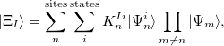
A fairly old idea for treating the excited states of a broad and highly relevant class of weakly interacting molecular aggregates is the so called Frankel-Davydov Exciton model. In such a model the excited states of the total aggregate is treated as a linear combination of excitations that are localized on molecular sites; the $I$ th excited state, $|\Xi _ I\rangle$ , can be written,

$\begin{equation} |\Xi _ I\rangle =\sum _ n^{\rm sites} \sum _ i^{\rm states} K_ n^{Ii} |\Psi _ n^ i\rangle \prod _{m\neq n}|\Psi _ m\rangle , \end{equation}$

(12.24)

where $|\Psi _ n^ i\rangle$ is the $i$ th excited state of the $n$ th molecular fragment and when un-superscripted corresponds to the ground state of the same. Eigenstates and energies are found by computing the electronic Hamiltonian matrix in this direct product, exciton-site basis and diagonalizing it. The AIFDEM[789] approach is an ab-initio realization of this ansatz whereby the exciton-site basis is compromised of direct products of ab-initio wave functions that are computed for the isolated fragments. Fragment ground states are described by single SCF determinants, $\Phi _{\! A}$ , and fragment excited states are linear combinations of singly-excited determinants,

$\begin{equation} |\Psi _{\! A}^\ast \rangle = \sum _{ia} C^{ia}|\Phi _{\! A}^{ia}\rangle . \end{equation}$

(12.25)

The AIFDEM approach computes elements of the Hamiltonian,

$\begin{equation} \label{eq:AIFDEM_ H} \langle \Psi _{\! A}^\ast \Psi _{\! B}\Psi _{\! C}\ldots |\hat{H}|\Psi _{\! A}\Psi _{\! B}^\ast \Psi _{\! C}\ldots \rangle = \sum _{ia \sigma }\sum _{kb \tau } C^{i a }_{\sigma } C^{kb}_{\tau }\langle \Phi ^{ia}_{\! A}\Phi _{\! B} \Phi _{\! C}\ldots |\hat{H}|\Phi _{\! A}\Phi ^{k b}_{\! B}\Phi _{\! C}\ldots \rangle \; , \end{equation}$

(12.26)

and overlap matrices,

$\begin{equation} \label{eq:AIFDEM_ S} \left\langle \Psi _{\! A}^\ast \Psi _{\! B}\Psi _{\! C}\ldots |\Psi _{\! A}\Psi _{\! B}^\ast \Psi _{\! C} \ldots \right\rangle = \sum _{ia \sigma }\sum _{kb \tau } C^{i a}_{\sigma } C^{kb}_{\tau } \langle \Phi ^{ia}_{\! A}\Phi _{\! B}\Phi _{\! C}\ldots |\Phi _{\! A}\Phi ^{k b}_{\! B}\Phi _{\! C}\ldots \rangle \; . \end{equation}$

(12.27)

The fragment excited states are transformed into the NTO basis, see section 6.12.2, to minimize the number of terms in the expansions and the corresponding orbitals transformation, see section 10.16.2.2, is utilized to compute the matrix elements of the non-orthogonal orbitals for each term in the RHS of equations eq:AIFDEM_H and eq:AIFDEM_S. The eigenstates and eigenenergies of the exciton Hamiltonian are printed and saved to a scratch file; transition dipole moments between the ground and first ten exciton eigenstates are also computed.

The cost to compute each matrix element scales as the size of the supersystem, approximately $\mathcal{O}\left(N^{2-4}\right)$ , since all fragments must be included in the direct products in equations eq:AIFDEM_H and eq:AIFDEM_S. To reduce this scaling a physically motivated charge embedding scheme was recently introduced [790] that only treats the excited fragments, and neighbors within a user specified distance threshold, with full QM while the other ground state fragment interactions are approximated by point charges. Point charge type is specified using the XPOL_CHARGE_TYPE keyword. In general, the inclusion of neighboring fragments in the QM part of the matrix element evaluation does not seem to significantly improve the accuracy and diminishes the cost savings of the charge embedding procedure. Therefore, the minimal “ 0 ” threshold, where only the excited fragments are treated with QM, can be considered optimal. Charge embedding with the minimal threshold affords and algorithm that scales as $F^2 \times \mathcal{O}\left(n_{pair}^{2-4}\right)$ , where $F$ is the number of fragments and $n_{pair}$ is the size of a pair of fragments.

The exciton-site basis can be expanded to include higher lying fragment excited states which gives the wave function variational flexibility and can significantly improve accuracy for polar systems and delocalized excited states. The number of fragment excited states to include in the basis is specified by the CIS_N_ROOTS keyword (should be equal to 1 at minimum). A cost effective means of including polarization effects is to utilize the XPol method to compute fragment ground states, see section 12.7 and associated job controls, fragment excited states are then computed using the XPol polarized MOs. Charge transfer-like states of the form, $|\Phi _{\! A}^+\Phi _{\! B}^-\Phi _{\! C}\ldots \rangle$ , where $\Phi _{\! A}^{ + \left( - \right)}$ represent cation (anion) determinants from unrestricted SCF calculations on the isolated fragments, can also be included in the basis.

The exciton-site basis states are spin adapted, their multiplicity determines that of the target excited state and this must be specified by setting CIS_SINGLETS or CIS_TRIPLETS to TRUE. The number of terms that are included in equations eq:AIFDEM_H and eq:AIFDEM_S can be rationally truncated at some fraction of the norm of the fragment NTO amplitudes to reduce computational cost at the expense of some accuracy. Computation time scales approximately quadratically with the number of these terms and a threshold of about 85% has been found to maintain acceptable accuracy for organic molecules with reasonable cost. The fragment orbitals and excited states may be computed with any level of SCF and single excitation theory, including DFT and TDDFT, however the coupling matrix elements are always computed with a CIS-like Hamiltonian with no DFT exchange-correlation. Both OpenMP, and MPI parallel implementations are available; the former distributes two-electron integral computation across cores in a node as in a traditional excited state calculation, the latter can distribute matrix element evaluations across hundreds of cores with minimal overhead.

12.11.2 Job Control for AIFDEM

AIFDEM

Perform an AIFDEM calculation.

TYPE:

LOGICAL

DEFAULT:

FALSE

OPTIONS:

FALSE

Do not perform an AIFDEM calculation.

TRUE

Perform an AIFDEM calculation.

RECOMMENDATION:

False

AIFDEM_NTOTHRESH

Controls the number of NTOs that are retained in the exciton-site basis states.

TYPE:

INTEGER

DEFAULT:

99

OPTIONS:

$n$

Threshold percentage of the norm of fragment NTO amplitudes.

RECOMMENDATION:

A threshold of $85 \%$ gives a good tradeoff of computational time and accuracy for organic molecules.

AIFDEM_EMBED_RANGE

Specifies the size of the QM region for charge embedding

TYPE:

INTEGER

DEFAULT:

FULL_QM

OPTIONS:

FULL_QM

No charge embedding.

0

Treat only excited fragments with QM.

$n$

Range () from excited fragments within which to treat other fragments with QM.

RECOMMENDATION:

Minimal, 0 , threshold maintains accuracy while significantly reducing computational time.

AIFDEM_CTSTATES

Include charge-transfer-like cation/anion pair states in the AIFDEM basis.

TYPE:

LOGICAL

DEFAULT:

FALSE

OPTIONS:

TRUE

Include CT states.

FALSE

Do not include CT states.

RECOMMENDATION:

None

Example 12.289 Example showing singlet excited state calculation, on (H $_2$ O) $_4$ . XPol is used to generate monomer wave functions with ChElPG charges. Minimal QM charge embedding is used for the exciton model with three excited states per fragment.



$rem
BASIS  =  aug-cc-pvdz
EXCHANGE  =  HF
CIS_N_ROOTS = 3
CIS_TRIPLETS = FALSE
XPOL TRUE
XPOL_CHARGE_TYPE QCHELPG
AIFDEM  TRUE
AIFDEM_EMBED_RANGE = 0
AIFDEM_NTOTHRESH = 90
NTO_PAIRS  1
$end

$molecule
0 1
--H2O 0
0 1
O          1.74078        1.59716       -1.49814
H          2.22908        2.18316       -2.08914
H          0.88038        2.04726       -1.32684
--H2O 1
0 1
O          1.31998       -1.18934       -1.91734
H          1.49988       -0.22974       -1.89044
H          1.69058       -1.52594       -1.07704
--H2O 2
0 1
O         -0.68982        2.59476       -0.72224
H         -1.14372        3.37086       -1.07364
H         -1.35592        1.84986       -0.78334
--H2O 3
0 1
O         -1.27512       -1.77394       -1.69524
H         -0.32252       -1.52884       -1.85604
H         -1.53992       -2.30454       -2.45644
$end

FALSE	Do not perform an AIFDEM calculation.
TRUE	Perform an AIFDEM calculation.

FULL_QM	No charge embedding.
0	Treat only excited fragments with QM.
$n$	Range () from excited fragments within which to treat other fragments with QM.